The Simplest Way Machines Learn — Finding Friends in a Crowd

Machine-Learning tutorial · PySpark.in

Making "Why Machines Learn" easy for everyone

Have you ever walked into a party and spotted your friend just by looking at the people standing closest to you? You did not measure their nose length or count their freckles. You just thought, "That person looks like my friend, so it probably is my friend."

Believe it or not, this simple idea — "if they look alike, they probably are alike" — is one of the most powerful tricks in Machine Learning. It is called the Nearest Neighbor rule, and it is so simple that you might wonder if it even counts as "learning." But as Anil Ananthaswamy shows in his book Why Machines Learn, this humble idea changed the history of AI.

1. From Pictures to Long Lists of Numbers

Before a machine can learn, we must teach it how to "see" the world. The book starts with a beautiful example. Imagine a small digital screen with 7 rows and 9 columns — like a tiny calculator display. That gives us 63 tiny squares (pixels).

Now, imagine drawing the number 2 on this screen. Some squares turn black, others stay white. If we write 1 for every black square and 0 for every white square, we get a list of 63 numbers:

[0, 1, 1, 1, 1, 1, 1, 1, 0,

0, 0, 0, 0, 0, 0, 0, 1, 0,

0, 0, 0, 0, 0, 0, 1, 0, 0,

... ] (63 numbers total)

This list is not just a list. In mathematics, it is a vector — an arrow pointing to a specific location in space. Because there are 63 numbers, we say this is a point in 63-dimensional space.

Yes, 63 dimensions! It sounds like science fiction, but it is just a fancy way of saying "63 different directions." Your everyday 3D world has X, Y, and Z. Our number image has direction 1, direction 2, all the way to direction 63.

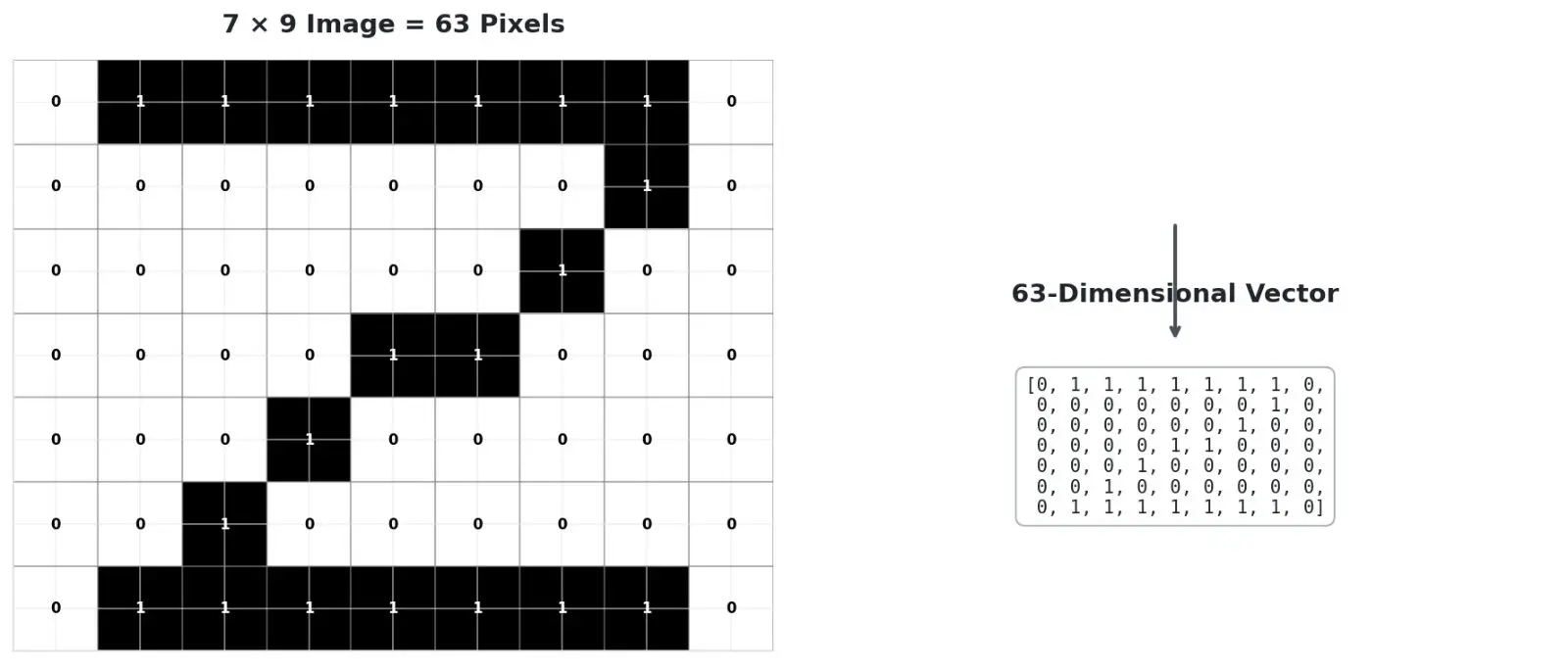
Figure 1: A simple 7×9 image becomes a list of 63 numbers — a vector living in 63-dimensional space.

If ten different people draw the number 2, each drawing will be slightly different. But because everyone draws "2" roughly the same way, all those 63-number vectors will cluster together in that giant 63D space. The same happens for the number 8, but in a different cluster.

So here is the magic question: If we get a new drawing, how do we know if it is a 2 or an 8?

The answer is almost too simple: find the closest known drawing and copy its label.

2. The Caveman Rule

Ananthaswamy tells us that mathematicians Evelyn Fix and Joseph Hodges wrote the first technical report about this idea in 1951, at an Air Force base in Texas. Later, a graduate student named Peter Hart at Stanford found their paper. He was fascinated.

Hart teamed up with a young professor named Thomas Cover. Together, they proved something amazing: even though the Nearest Neighbor rule seems almost childish, its accuracy has strict mathematical limits. In fact, as you collect more and more data, this simple rule gets surprisingly close to the best possible classifier in the world (the "Bayes optimal" classifier).

Peter Hart described the rule as "caveman intuition": If they look alike, they probably are alike.

Here is how it works step by step:

Store all your labeled examples (the "training data").
When a new example arrives, measure its distance to every stored example.
Find the closest one — the "nearest neighbor."
Give the new example the same label as that neighbor.

That's it. No complex formulas. No training phase where the machine "adjusts" itself. Just distance and copying.

3. Why Simple Can Be Better Than Smart

Now, you might think, "Surely a straight line is better than this?" After all, many algorithms try to draw a line between two groups.

Ananthaswamy shows us a classic example in the book: a group of gray circles and black triangles scattered on a page. The tricky part? They are mixed together. There is no single straight line that can separate them perfectly. A simple line-drawing algorithm like the Perceptron will fail here.

But the Nearest Neighbor algorithm doesn't draw straight lines. It draws a squiggly, organic boundary that wraps around the data like a shoreline around islands.

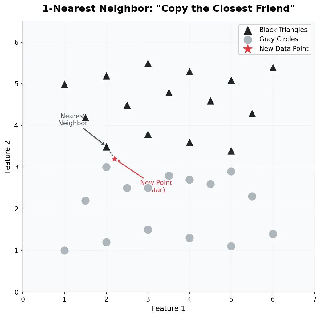
Figure 2: Gray circles and black triangles that no straight line can separate. The star is a new data point. The 1-Nearest Neighbor rule finds the closest shape and copies its label.

Look at the star in the image above. Is it a circle or a triangle? The nearest neighbor algorithm just measures distance. If the closest shape is a circle, the star becomes a circle. The result is a natural, curved boundary between the two teams.

4. When Simple Becomes Too Simple: The Overfitting Trap

But wait. If one neighbor is good, isn't one neighbor too good?

Imagine one lonely black triangle accidentally landed in the middle of a big group of gray circles. Maybe a human mislabeled it. Maybe it is just a weird outlier.

If our algorithm trusts only the single nearest neighbor, it will create a tiny "island" around that lone triangle. Any new point falling near that island will be called a triangle, even though it is surrounded by circles. The algorithm is being too obedient to the training data. It memorizes every quirk and mistake.

In Machine Learning, this is called overfitting. The algorithm fits the training data so tightly that it captures noise, not truth.

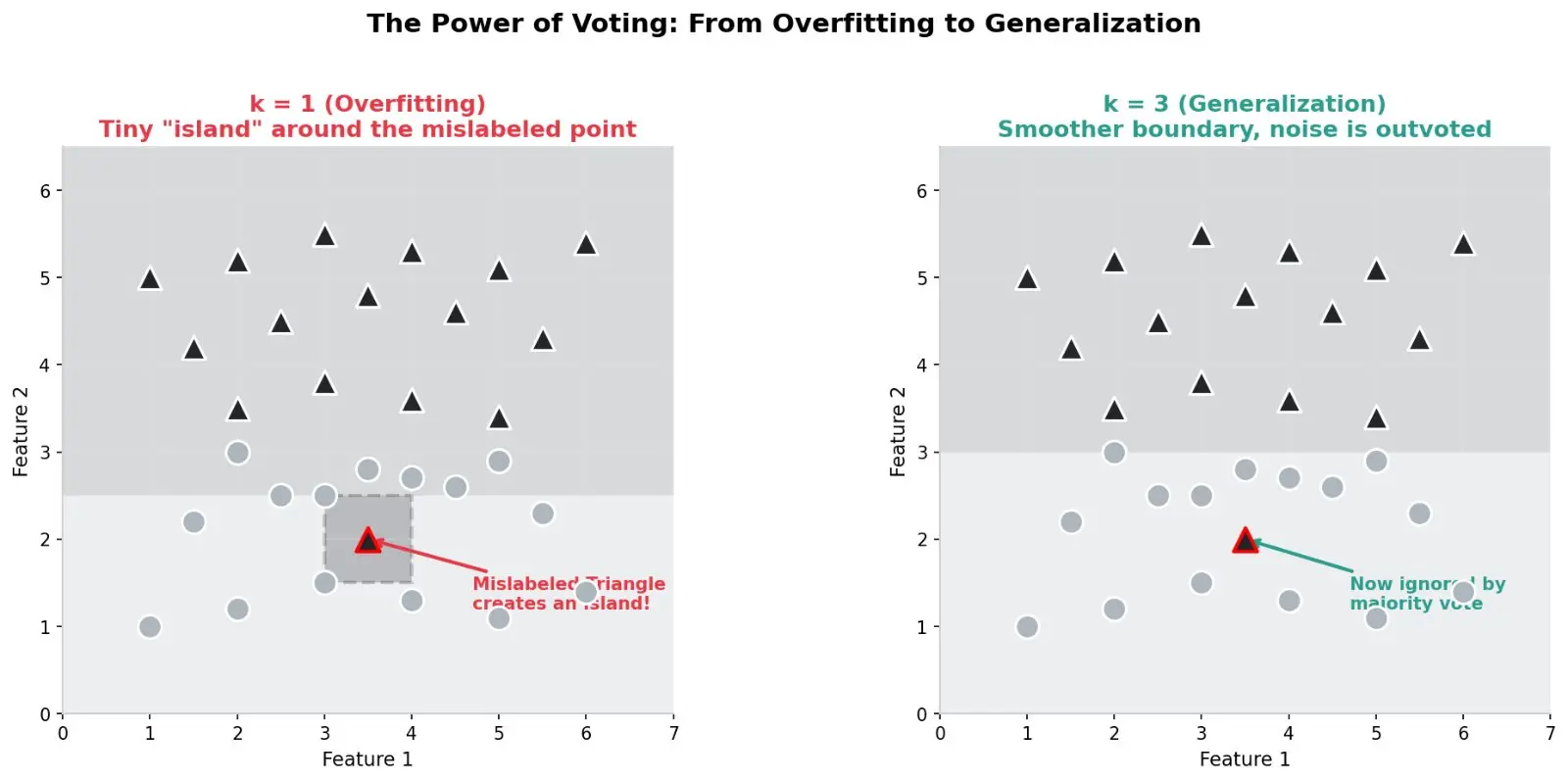
Figure 3: Left: 1-Nearest Neighbor creates a tiny island around a mislabeled triangle. Right: Using 3 neighbors smooths the boundary and ignores the noise.

5. The Fix: Ask a Committee, Not One Person

The solution is elegant and democratic: instead of asking the single closest neighbor, ask the K closest neighbors and take a majority vote.

If K = 3, we find the three nearest shapes. If two are circles and one is a triangle, we call the new point a circle. The triangle is outvoted.

Why do we usually pick an odd number like 3, 5, or 7? To avoid ties. If you ask 2 neighbors and one says "circle" while the other says "triangle," you are stuck. An odd number guarantees a decision.

As K grows larger, the boundary becomes smoother. The algorithm stops caring about every single outlier. It starts seeing the big picture. This is called generalization — the ability to handle new, unseen data wisely.

Of course, there is a trade-off. If K is too large, the algorithm might become too lazy and blur the boundary so much that it misclassifies some correct training points. Finding the right K is an art.

6. Let's Build It With Bare Hands: Python from Scratch

To truly understand k-NN, let's write it without any fancy Machine Learning libraries. We will use only plain Python and a small dataset of 2D points.

Imagine we have two types of fruits measured by weight and sweetness:

Apples (label 0): (150g, 7/10 sweetness), (170g, 8/10), (140g, 6/10)
Oranges (label 1): (180g, 9/10), (200g, 8/10), (190g, 9/10)

We get a new fruit: (160g, 7/10). Is it an apple or an orange?

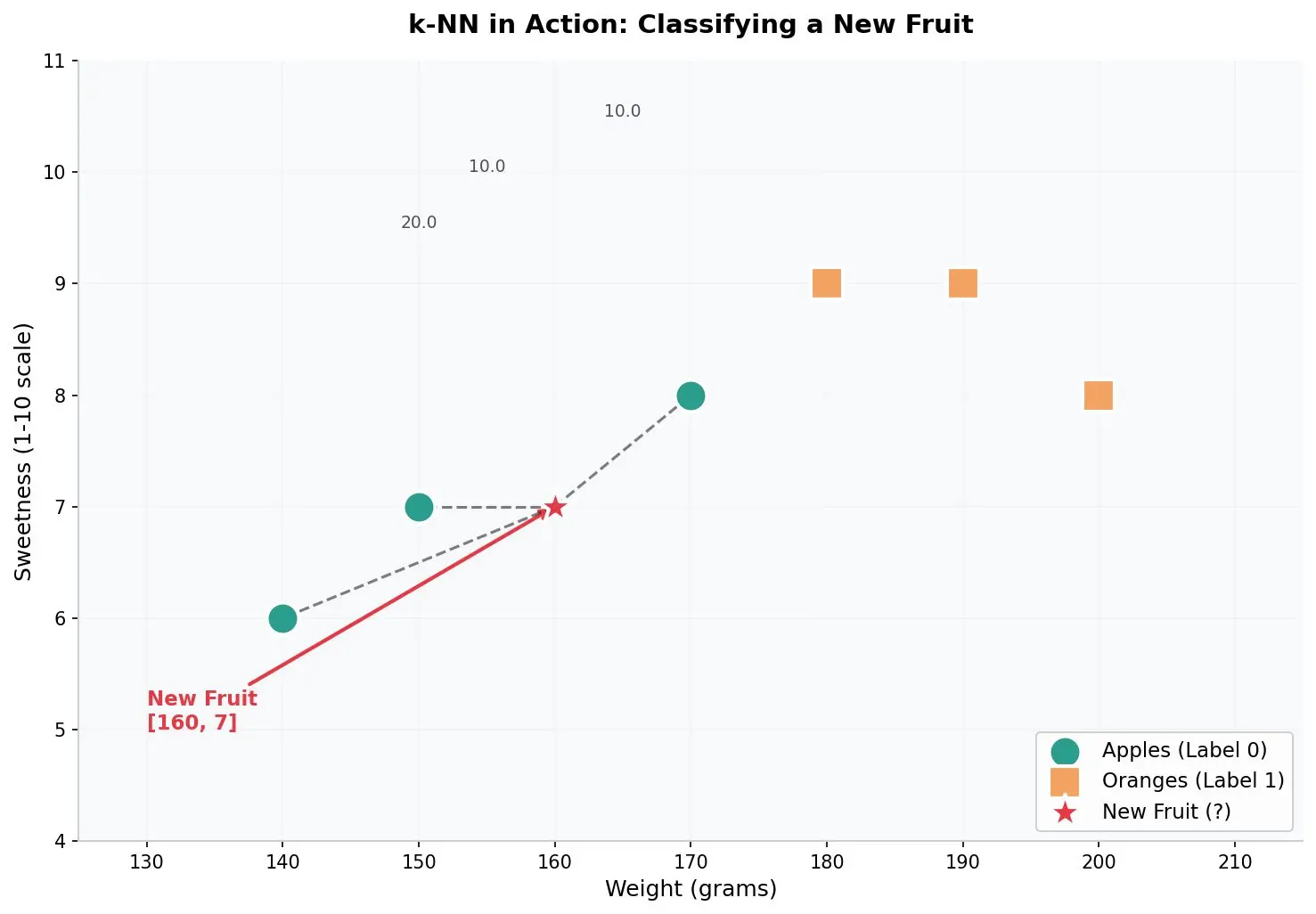
Figure 4: Our tiny fruit dataset. The new fruit (red star) is closest to the apple team.

Here is the complete code, using nothing but basic Python:

```

python

import math

# Training data: [weight, sweetness, label]

# Label 0 = Apple, Label 1 = Orange

training_data = [

[150, 7, 0],

[170, 8, 0],

[140, 6, 0],

[180, 9, 1],

[200, 8, 1],

[190, 9, 1]

]

def euclidean_distance(point1, point2):

"""Calculate straight-line distance between two points."""

total = 0

for i in range(len(point1)):

total += (point1[i] - point2[i]) ** 2

return math.sqrt(total)

def knn_predict(new_point, data, k=3):

"""Predict the label of new_point using k-Nearest Neighbors."""

# Step 1: Calculate distance to every training point

distances = []

for row in data:

features = row[:-1] # all except last column

label = row[-1] # last column is label

dist = euclidean_distance(new_point, features)

distances.append((dist, label))

# Step 2: Sort by distance (closest first)

distances.sort(key=lambda x: x[0])

# Step 3: Take the first k neighbors and vote

votes = {}

for i in range(k):

label = distances[i][1]

votes[label] = votes.get(label, 0) + 1

# Step 4: Return the label with most votes

best_label = max(votes, key=votes.get)

return best_label, distances[:k]

# New fruit to classify

new_fruit = [160, 7]

# Try with k=1 and k=3

for k in [1, 3]:

prediction, neighbors = knn_predict(new_fruit, training_data, k=k)

fruit_name = "Apple" if prediction == 0 else "Orange"

print(f"\nWith k={k}:")

print(f" Predicted: {fruit_name}")

print(f" Neighbors considered: {len(neighbors)}")

for dist, lbl in neighbors:

name = "Apple" if lbl == 0 else "Orange"

print(f" - Distance {dist:.2f} -> {name}")

```

Output:

With k=1:

Predicted: Apple

Neighbors considered: 1

- Distance 10.00 -> Apple

With k=3:

Predicted: Apple

Neighbors considered: 3

- Distance 10.00 -> Apple

- Distance 14.14 -> Apple

- Distance 22.36 -> Orange

Even with just basic math, the algorithm works! It found that the new fruit is closer to the apple team. Notice how with k=3, it still says "Apple" because two out of three nearby fruits are apples.

7. The Beautiful Math Behind the Simplicity

You might wonder: can something this simple really compete with super-complex algorithms?

Peter Hart and Thomas Cover proved that it can. They showed that as your dataset grows very large, the k-NN algorithm (with a well-chosen K) approaches the performance of the Bayes Optimal Classifier — the theoretical perfect classifier that knows the true probability distributions behind the data.

The book shows a beautiful graph comparing the error rate of the Bayes classifier (the dashed line) against the Nearest Neighbor risk (the solid curve). As K increases and the dataset grows, the curve flattens and hugs the dashed line.

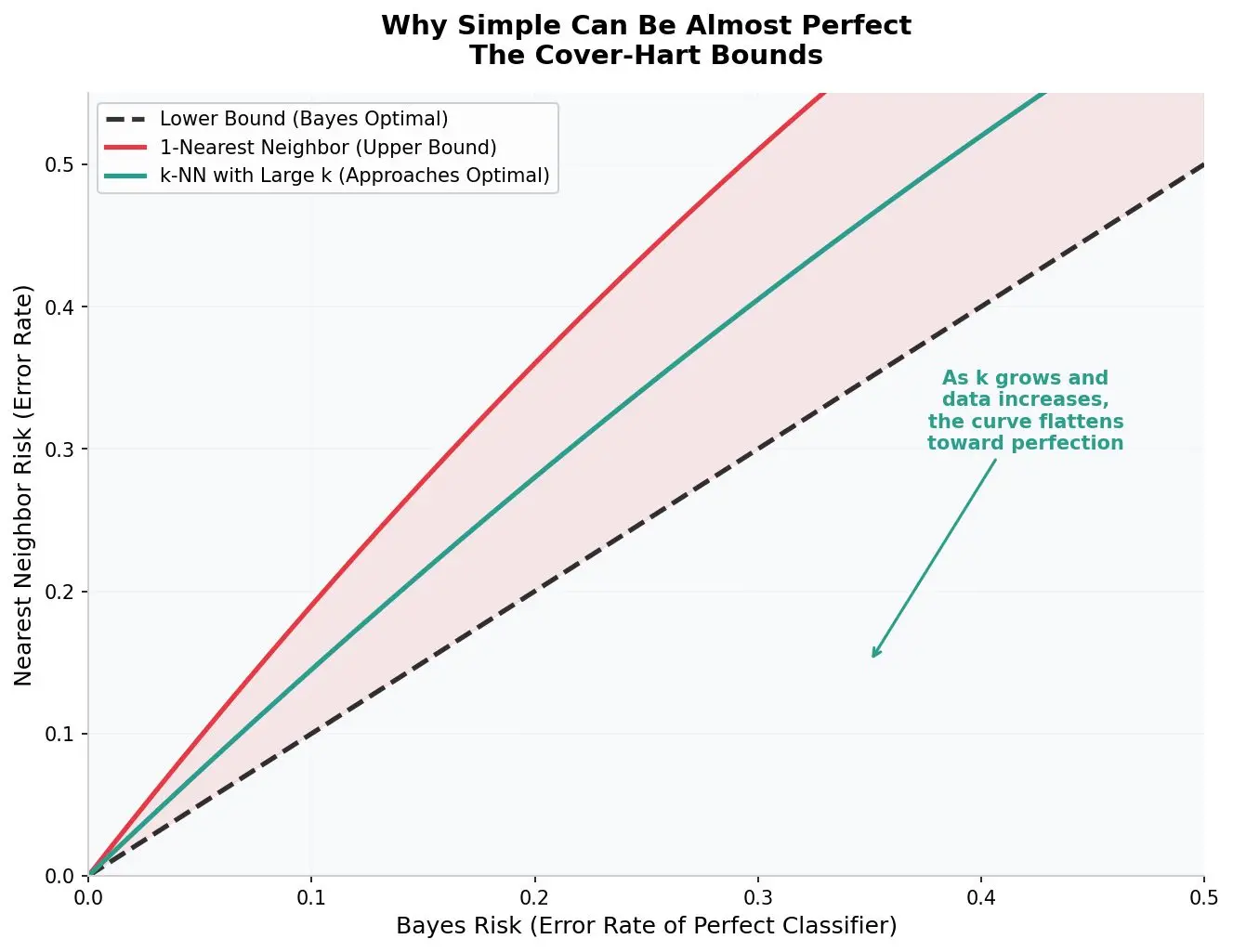
Figure 5: The k-NN error rate (solid curves) approaches the unbeatable Bayes optimal error rate (dashed line) as data grows.

However, there is a price to pay. k-NN is what mathematicians call a nonparametric model. Unlike the Perceptron, which learns a small set of weights and forgets the training data, k-NN memorizes everything. It stores every single example. As datasets explode in size (think millions of images), k-NN becomes slow and hungry for memory.

There is also the Curse of Dimensionality. In very high-dimensional spaces (like our 63-pixel number example), distances start behaving strangely. Every point begins to feel equally far away, and the concept of "nearest" loses its meaning. Our human brains, built for 3D worlds, are simply not equipped to imagine this weirdness.

8. Why This Matters for You

The Nearest Neighbor rule teaches us a profound lesson: sometimes the simplest idea is the deepest.

You don't need neural networks with billions of parameters to start understanding Machine Learning. You need the intuition that patterns live as points in space, and closeness means similarity. This idea powers recommendation engines ("people like you bought this book"), medical diagnosis ("patients with similar symptoms had this disease"), and even how fruit flies smell flowers.

As Ananthaswamy beautifully puts it, the algorithm achieves something remarkable: it finds a nonlinear boundary to separate one class from another, without ever being explicitly told what that boundary should look like.

Reference

Ananthaswamy, Anil. Why Machines Learn: The Elegant Math Behind Modern AI. Dutton, 2024.