The First Artificial Neuron and Learning from Mistakes

Machine-Learning tutorial · PySpark.in

1. The Problem We Are Solving

We know how biological neurons work — they receive signals, process them, and fire when enough input is received. We also know that early computing machines could perform logic but could not adapt. Now we put these two ideas together and answer the most important question in machine learning:

Given examples of data with correct answers, can we build a machine that learns from its mistakes and improves over time?

The answer is elegant and comes in two pieces. First, build a simple mathematical model of a neuron — we call this the McCulloch-Pitts neuron. Second, add a learning rule that adjusts the model when it makes mistakes. The total collection is the perceptron, the first machine that could truly learn.

Complete idea: Artificial Neuron + Learning Rule = Machine Learning

2. Why This Story Matters

The logic is simple. If we can model how a brain cell computes, and then teach that model to correct its own errors, then:

Biological inspiration + Mathematical rigor + Learning from data = Modern AI

So every vector of the form "neuron + adjustment" is indeed a learning system. Conversely, if any machine can learn from examples, then it must have both components — a computing unit and a way to update that unit based on mistakes. Every modern AI system is captured by our formula. The complete picture is exactly the right-hand side shift from fixed logic to adaptive learning: we take the artificial neuron and add the ability to change its weights based on error.

Historical picture: the McCulloch-Pitts neuron (1943) was a fixed computational device passing through strict logic. The complete solution to machine learning is the same shape — same neuron structure — but shifted so that its weights pass through learned values instead of hand-engineered ones. Mathematicians and computer scientists call this a perceptron or adaptive linear neuron.

3. Finding the First Artificial Neuron

To find the McCulloch-Pitts model, we look at how real brain cells work and simplify. The real neuron has three main parts — dendrites that receive, a cell body that processes, and an axon that sends signals. Setting this to the simplest possible mathematical form gives one particular model without any learning ability.

Let us work through the full story. Take two unlikely collaborators:

Warren McCulloch — An American neurophysiologist in his mid-forties, trained in philosophy, psychology, and medicine. During the 1930s, he mapped monkey brain connectivity and obsessed over the "logic of the brain."

Walter Pitts — A homeless teenage prodigy, already an accomplished logician and protégé of the mathematician Rudolf Carnap. He was attending seminars by the Ukrainian mathematical physicist Nicolas Rashevsky in Chicago.

McCulloch moved from Yale to the University of Illinois in 1941, where he met Pitts. McCulloch and his wife, Rook, gave Walter a home. As computer scientist Michael Arbib wrote: "There followed endless evenings sitting around the McCulloch kitchen table trying to sort out how the brain worked, with the McCullochs' daughter Taffy sketching little pictures." Taffy's drawings would later illustrate their 1943 paper, "A Logical Calculus of the Ideas Immanent in Nervous Activity."

In that work, McCulloch and Pitts proposed a simple model of a biological neuron:

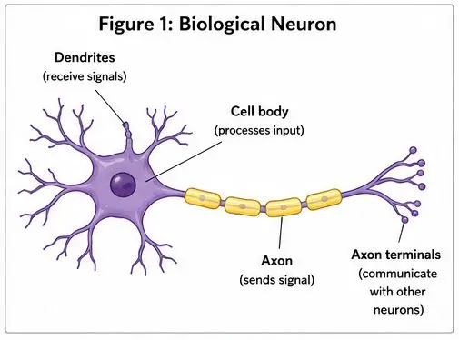
The neuron's cell body receives inputs via its treelike projections, called dendrites. The cell body performs some computation on these inputs. Then, based on the results of that computation, it may send an electrical signal spiking along another, longer projection, called the axon. That signal travels along the axon and reaches its branching terminals, where it's communicated to the dendrites of neighboring neurons.

McCulloch and Pitts turned this into a simple computational model, an artificial neuron, or neurode (for "neuron" + "node"):

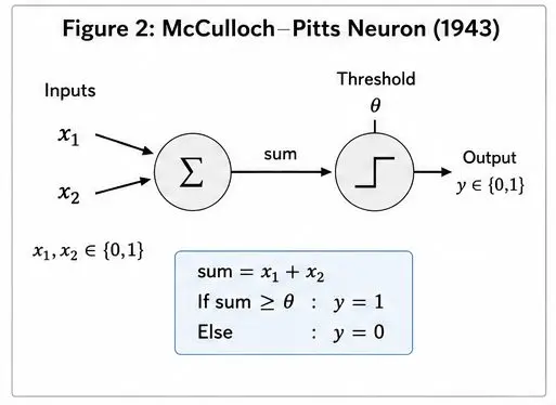
In this simple version of the McCulloch-Pitts model, x₁ and x₂ can be either 0 or 1. In formal notation:

x₁, x₂ ∈ {0,1}

That should be read as: x₁ is an element of the set {0, 1} and x₂ is an element of the set {0, 1}; x₁ and x₂ can take on only values 0 or 1 and nothing else. The neurode's output y is calculated by first summing the inputs and then checking to see if that sum is greater than or equal to some threshold, theta (θ). If so, y equals 1; if not, y equals 0.

sum = x₁ + x₂

If sum ≥ θ: y = 1

Else: y = 0

Generalizing this to an arbitrary sequence of inputs, we define the function g(x) — which sums up the inputs. Then we define the function f(g(x)) — which takes the summation and performs the thresholding to generate the output y:

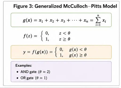
g(x) = x₁ + x₂ + x₃ + ... + xₙ = Σ xᵢ

f(z) = { 0, z < θ

{ 1, z ≥ θ

y = f(g(x)) = { 0, g(x) < θ

{ 1, g(x) ≥ θ

With one artificial neuron as described, we can design some of the basic Boolean logic gates (AND & OR, for example). In an AND logic gate, the output y should be 1 if both x₁ and x₂ are equal to 1; otherwise, the output should be 0. In this case, θ = 2 does the trick. Now, the output y will be 1 only when x₁ and x₂ are both 1.

For an OR gate, the output should be 1 if either x₁ or x₂ is 1; otherwise, the output should be 0. What should θ be? θ = 1.

The simple MCP model can be extended. You can increase the number of inputs. You can let inputs be "inhibitory," meaning x₁ or x₂ can be multiplied by −1. If one of the inputs to the neurode is inhibitory and you set the threshold appropriately, then the neurode will always output a 0, regardless of the value of all the other inputs. This allows you to build more complex logic.

All this was amazing, and yet limited. The McCulloch-Pitts (MCP) neuron is a unit of computation, and you can use combinations of it to create any type of Boolean logic. Given that all digital computation at its most basic is a sequence of such logical operations, you can essentially mix and match MCP neurons to carry out any computation. This was an extraordinary statement to make in 1943.

But the upshot was simply a machine that could compute, not learn. In particular, the value of θ had to be hand-engineered; the neuron couldn't examine the data and figure out θ.

4. The Complete Solution: Adding Learning

We already found the computing unit. Now we add the missing piece — the ability to learn from mistakes.

Enter Frank Rosenblatt, a young psychologist who synthesized the work of McCulloch, Pitts, and the Canadian psychologist Donald Hebb. Hebb had proposed in 1949 that biological neurons learn because connections between neurons strengthen when one neuron's output is consistently involved in the firing of another. This process is called Hebbian learning — often summarized as "Neurons that fire together wire together."

Rosenblatt took the work of these pioneers and synthesized it into a new idea: artificial neurons that reconfigure as they learn, embodying information in the strengths of their connections.

As a psychologist, Rosenblatt didn't have access to the kind of computer power he needed to simulate his ideas in hardware or software. So, he borrowed time on the Cornell Aeronautical Laboratory's IBM 704, a five-ton, room-size behemoth. Rosenblatt eventually built the Mark I Perceptron. The device had a camera that produced a 20×20-pixel image. The Mark I, when shown these images, could recognize letters of the alphabet.

But saying that the Mark I "recognized" characters is missing the point. As George Nagy, Rosenblatt's student, would say in his talks: "The point is that Mark I learned to recognize letters by being zapped when it made a mistake!"

In its simplest form, a perceptron is an augmented McCulloch-Pitts neuron imbued with a learning algorithm:

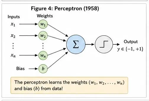
Note that each input is being multiplied by its corresponding weight. There is also an extra input, b, the bias.

The computation carried out by the perceptron goes like this:

sum = w₁x₁ + w₂x₂ + b

If sum > 0: y = 1

Else: y = −1

More generally and in mathematical notation:

g(x) = w₁x₁ + w₂x₂ + ... + wₙxₙ + b = Σ wᵢxᵢ + b

f(z) = { −1, z ≤ 0

{ 1, z > 0

y = f(g(x)) = { −1, g(x) ≤ 0

{ 1, g(x) > 0

The main difference from the MCP model presented earlier is that the perceptron's inputs don't have to be binary (0 or 1), but can take on any value. Also, these inputs are multiplied by their corresponding weights, so we now have a weighted sum. Added to that is an additional term b, the bias. The output, y, is either −1 or +1 (instead of 0 or 1, as in the MCP neuron).

Crucially, unlike with the MCP neuron, the perceptron can learn the correct value for the weights and the bias for solving some problem.

5. A Real Example: Learning to Classify

To understand how this works, consider a perceptron that seeks to classify someone as obese, y = +1, or not-obese, y = −1. The inputs are a person's body weight, x₁, and height, x₂. Let's say that the dataset contains a hundred entries, with each entry comprising a person's body weight and height and a label saying whether a doctor thinks the person is obese according to guidelines set by the National Heart, Lung, and Blood Institute.

A perceptron's task is to learn the values for w₁ and w₂ and the value of the bias term b, such that it correctly classifies each person in the dataset as "obese" or "not-obese."

Once the perceptron has learned the correct values for w₁ and w₂ and the bias term, it's ready to make predictions. Given another person's body weight and height — this person was not in the original dataset — the perceptron can classify the person as obese or not-obese.

Of course, a few assumptions underlie this model. But the perceptron makes one basic assumption: It assumes that there exists a clear, linear divide between the categories of people classified as obese and those classified as not-obese.

In the context of this simple example, if you were to plot the body weights and heights of people on an xy graph, with weights on the x-axis and heights on the y-axis, such that each person was a point on the graph, then the "clear divide" assumption states that there would exist a straight line separating the points representing the obese from the points representing the not-obese. If so, the dataset is said to be linearly separable.

Here's a graphical look at what happens as the perceptron learns:

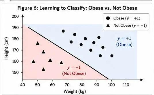
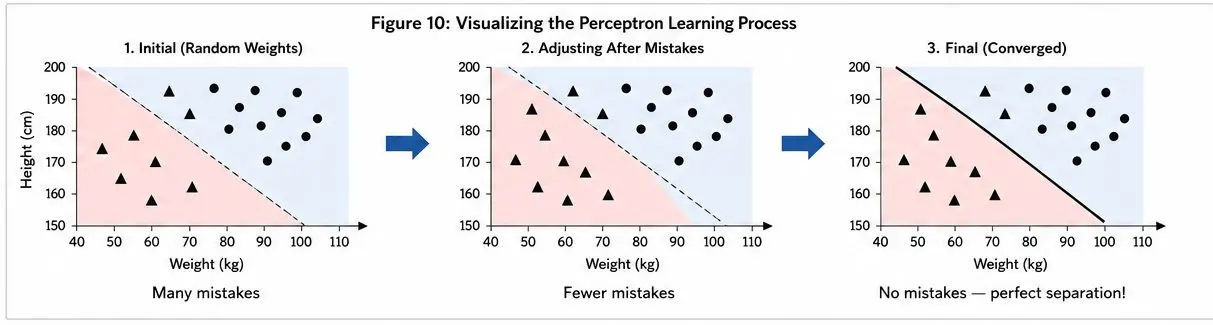
We start with two sets of data points, one characterized by black circles (y = +1, obese) and another by black triangles (y = −1, not-obese). Each data point is characterized by a pair of values (x₁, x₂), where x₁ is the body weight of the person in kilograms, plotted along the x-axis, and x₂ is the height in centimeters, plotted along the y-axis.

The perceptron starts with its weights, w₁ and w₂, and the bias initialized to zero. The weights and bias represent a line in the xy plane. The perceptron then tries to find a separating line, defined by some set of values for its weights and bias, that attempts to classify the points. In the beginning, it classifies some points correctly and others incorrectly.

Two of the incorrect attempts are shown as the gray dashed lines. In one attempt, all the points lie to one side of the dashed line, so the triangles are classified correctly, but the circles are not; and in another attempt, it gets the circles correct but some of the triangles wrong.

The perceptron learns from its mistakes and adjusts its weights and bias. After numerous passes through the data, the perceptron eventually discovers at least one set of correct values of its weights and its bias term. It finds a line that delineates the clusters: The circles and the triangles lie on opposite sides. This is shown as a solid black line separating the coordinate space into two regions (one of which is shaded gray).

The weights learned by the perceptron dictate the slope of the line; the bias determines the distance, or offset, of the line from the origin.

Once the perceptron has learned the correlation between the physical characteristics of a person (body weight and height) and whether that person is obese (y = +1 or −1), you can give it the body weight and height of a person whose data weren't used during training, and the perceptron can tell you whether that person should be classified as obese.

6. The Four Cases: Dimension Determines Everything

Given inputs of dimension n, there are important concepts to understand. The dimension determines both the complexity of the perceptron and the nature of the decision boundary.

Case 1: 2 Inputs — The Line

With two inputs (x₁, x₂), the perceptron finds a straight line to separate the data. We can visualize this easily on a 2D graph. The weights determine the slope, the bias determines the offset.

Example: Weight vs. Height classification

Case 2: 3 Inputs — The Plane

With three inputs (x₁, x₂, x₃), the data is three-dimensional. A line is no longer sufficient to separate the two clusters. You need a 2D plane to separate the data points.

Example: Weight, Height, and Age classification

Case 3: n Inputs — The Hyperplane

In dimensions of four or more, you need a hyperplane (which we cannot visualize with our 3D minds). In general, this higher-dimensional equivalent of a 1D straight line or a 2D plane is called a hyperplane.

Example: The Mark I Perceptron processed a 20×20-pixel image — for a total of 400 pixels, with each pixel corresponding to an x input value. So, the Mark I took as input a long row of values: x₁, x₂, x₃, ..., x₄₀₀.

Case 4: Non-Linearly Separable — The Limitation

If no straight line, plane, or hyperplane can separate the data, the single perceptron fails. This was the limitation that Marvin Minsky and Seymour Papert highlighted in 1969, causing the first "AI winter." The solution would later come from multi-layer networks.

Summary: The number of inputs n tells you the dimension of the space. The perceptron always finds a linear separator — a line in 2D, a plane in 3D, a hyperplane in n-D — if one exists. This is the master key to understanding the perceptron's power and its limitation.

7. Reading the Solution from the Perceptron

The perceptron algorithm makes everything explicit. After training on the data, the final weights and bias directly give you the decision boundary.

The learned weights form the normal vector to the separating hyperplane, and the bias tells you how far that hyperplane is from the origin. The decision boundary equation is:

w₁x₁ + w₂x₂ + ... + wₙxₙ + b = 0

This is why the perceptron learning rule is so powerful — it compresses all the work of finding the right weights into a single iterative process. The result is the 'answer key' for the whole classification problem.

To train a perceptron completely: (1) start with random weights and zero bias, (2) for each training example, make a prediction, (3) if wrong, update weights by w_new = w_old + learning_rate × true_label × input, (4) update bias by b_new = b_old + learning_rate × true_label, (5) repeat until no mistakes or maximum epochs reached.

Python Implementation: From Scratch

Below is a complete, zero-library implementation of both the McCulloch-Pitts neuron and the Perceptron. Run this code to see learning happen before your eyes.

```

python

# ============================================

# McCULLOCH-PITTS NEURON (1943) - Fixed Logic

# ============================================

class McCullochPittsNeuron:

"""

The first artificial neuron.

Inputs must be 0 or 1. Threshold is hand-engineered.

CANNOT learn from data.

"""

def __init__(self, threshold):

self.theta = threshold

def activate(self, inputs):

total = sum(inputs)

return 1 if total >= self.theta else 0

def __call__(self, inputs):

return self.activate(inputs)

print("=" * 50)

print("McCULLOCH-PITTS NEURON (1943)")

print("=" * 50)

# Truth table for 2 inputs

test_cases = [[0, 0], [0, 1], [1, 0], [1, 1]]

# AND GATE: Output is 1 ONLY if both inputs are 1

print("\n--- AND GATE (θ = 2) ---")

and_neuron = McCullochPittsNeuron(threshold=2)

for x in test_cases:

output = and_neuron(x)

print(f" Inputs: {x} | Sum: {sum(x)} | Output: {output}")

# OR GATE: Output is 1 if ANY input is 1

print("\n--- OR GATE (θ = 1) ---")

or_neuron = McCullochPittsNeuron(threshold=1)

for x in test_cases:

output = or_neuron(x)

print(f" Inputs: {x} | Sum: {sum(x)} | Output: {output}")

# NOT GATE (inhibitory input)

print("\n--- NOT GATE (inhibitory) ---")

def not_gate(x):

weighted_sum = (-1) * x[0]

return 1 if weighted_sum >= 0 else 0

for x in [[0], [1]]:

print(f" Input: {x} | Output: {not_gate(x)}")

# ============================================

# PERCEPTRON (1958) - The Learning Machine!

# ============================================

class Perceptron:

"""

Rosenblatt's Perceptron.

Learns weights and bias from data through mistakes.

"""

def __init__(self, num_inputs, learning_rate=0.01):

import random

random.seed(42)

self.weights = [random.uniform(-0.5, 0.5) for _ in range(num_inputs)]

self.bias = 0.0

self.learning_rate = learning_rate

self.history = []

def predict(self, inputs):

weighted_sum = sum(w * x for w, x in zip(self.weights, inputs)) + self.bias

return 1 if weighted_sum > 0 else -1

def train(self, training_data, max_epochs=100):

print(f"\nInitial weights: {[round(w, 3) for w in self.weights]}")

print(f"Initial bias: {self.bias}")

for epoch in range(max_epochs):

errors = 0

for inputs, true_label in training_data:

prediction = self.predict(inputs)

if prediction != true_label:

errors += 1

# The learning rule: adjust toward correct answer

for i in range(len(self.weights)):

self.weights[i] += self.learning_rate * true_label * inputs[i]

self.bias += self.learning_rate * true_label

self.history.append((self.weights.copy(), self.bias, errors))

print(f"Epoch {epoch + 1}: errors = {errors}, "

f"weights = {[round(w, 3) for w in self.weights]}, "

f"bias = {round(self.bias, 3)}")

if errors == 0:

print(f"\n🎉 Converged after {epoch + 1} epochs!")

break

return self.weights, self.bias

print("\n" + "=" * 60)

print("PERCEPTRON: LEARNING TO CLASSIFY OBESITY")

print("=" * 60)

# Training data: [weight_kg, height_cm] → obese (+1) or not (-1)

training_data = [

([50, 170], -1), ([55, 165], -1), ([60, 180], -1),

([45, 160], -1), ([70, 190], -1), # Not obese

([90, 160], 1), ([85, 155], 1), ([100, 170], 1),

([95, 165], 1), ([110, 175], 1), # Obese

]

perceptron = Perceptron(num_inputs=2, learning_rate=0.01)

weights, bias = perceptron.train(training_data, max_epochs=50)

print(f"\n{'='*60}")

print("FINAL LEARNED PARAMETERS:")

print(f" w1 (weight coefficient): {round(weights[0], 4)}")

print(f" w2 (height coefficient): {round(weights[1], 4)}")

print(f" b (bias): {round(bias, 4)}")

# Decision boundary: w1*x1 + w2*x2 + b = 0

# => x2 = -(w1/w2)*x1 - (b/w2)

slope = -weights[0] / weights[1]

intercept = -bias / weights[1]

print(f"\nDecision boundary: Height = {round(slope, 2)} × Weight + {round(intercept, 2)}")

# Test on new people

print(f"\n{'='*60}")

print("TESTING ON NEW PEOPLE:")

test_people = [([65, 175], "Not Obese"), ([88, 162], "Obese"),

([52, 168], "Not Obese"), ([105, 172], "Obese")]

for inputs, expected in test_people:

pred = perceptron.predict(inputs)

status = "Obese" if pred == 1 else "Not Obese"

print(f" Weight: {inputs[0]}kg, Height: {inputs[1]}cm → {status}")

```

Visualizing the Learning Process

The perceptron's journey from random guesses to perfect classification can be visualized as finding the right line through trial and error:

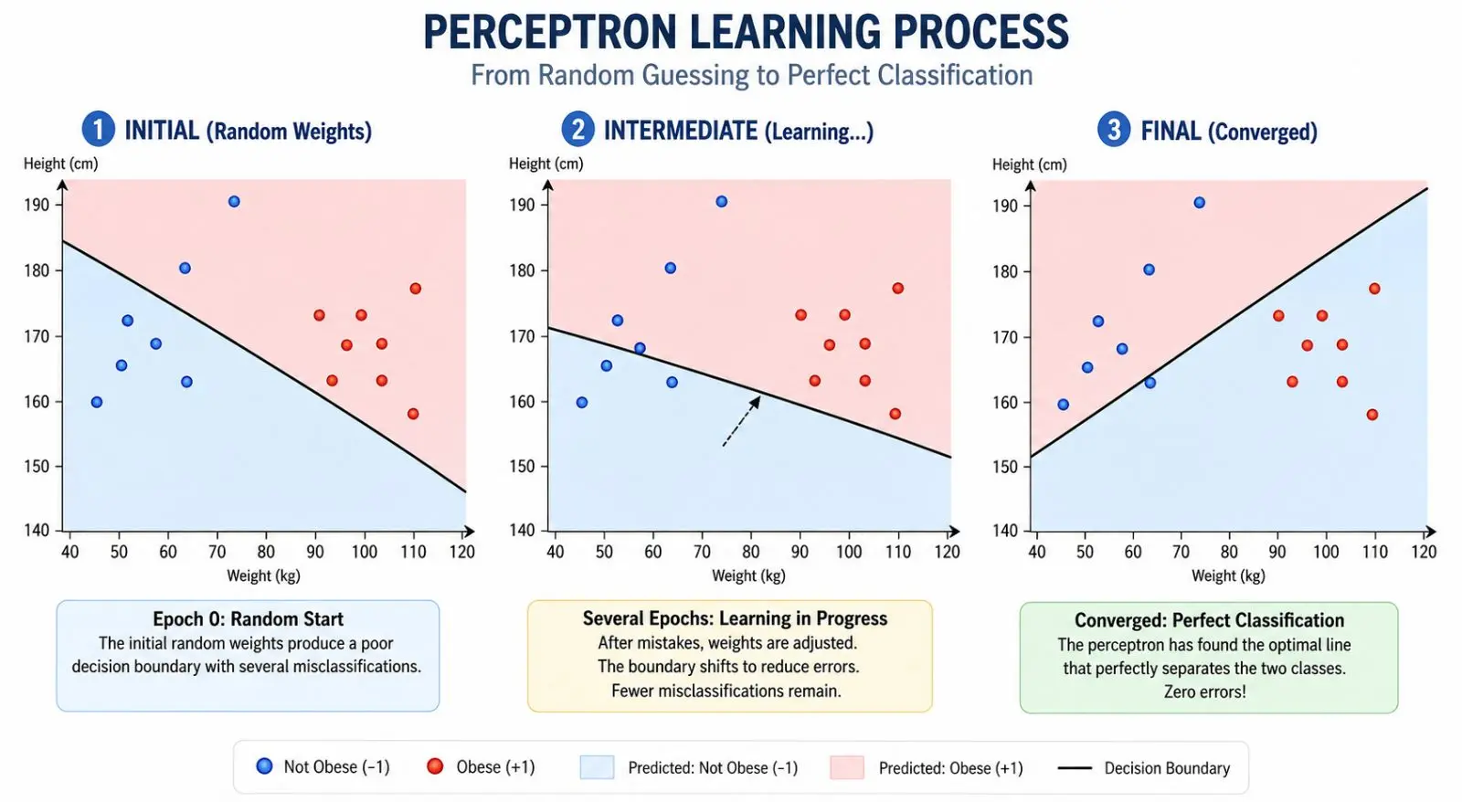
Left: Initial random weights create a wrong boundary. Middle: Adjusting after mistakes. Right: Final converged line perfectly separates the data. The shaded region shows the classification decision.

The Four Cases: Rank Determines Everything

Table

Complete solution = fixed artificial neuron + learning rule that updates weights based on mistakes. The shape and dimension come from the number of inputs. The location (shift from origin) comes from the learned bias.

Why the Perceptron Was Revolutionary

The McCulloch-Pitts neuron proved that machines could compute logical operations. But the perceptron proved something far more important: machines could learn from experience.

Rosenblatt built the Mark I Perceptron with numerous such units. It could process a 20×20-pixel image — for a total of 400 pixels. A complex arrangement of artificial neurons, both with fixed, random weights and weights that could be learned, turned this vector of 400 values into an output signal that could discern the pattern in the image.

But if you closely examine what the perceptron learns, its limitations — in hindsight, of course — become obvious. The algorithm is helping the perceptron learn about correlations between values of (x₁, x₂, ..., x₄₀₀) and the corresponding value of y. Sure, it learns the correlations without being explicitly told what they are, but these are correlations nonetheless.

Is identifying correlations the same thing as thinking and reasoning? Surely, if the Mark I distinguished the letter "B" from the letter "G," it was simply going by the patterns and did not attach any meaning to those letters that would engender further reasoning.

Such questions are at the heart of the modern debate over the limits of deep neural networks, the astonishing descendants of perceptrons. There is a path connecting these early perceptrons to the technology of large language models or the AI being developed for self-driving cars. That path is not a straight one; rather, it's long and winding, with false turns and dead ends. But it's a fascinating, intriguing path nonetheless, and we are setting off on it now.

Building the perceptron device was a major accomplishment. An even bigger achievement was the mathematical proof that a single layer of perceptrons will always find a linearly separating hyperplane, if the data are linearly separable.

References & Further Reading

Anil Ananthaswamy. Why Machines Learn: The Elegant Math Behind Modern AI. Dutton, 2024.

More Machine-Learning tutorials

• Introduction to Machine Learning
• Introduction to Deep Learning
• ​A Beginner's Guide to Machine Learning
• ​Patterns
• ​ Understanding Vectors, the Building Blocks of AI
• How Vectors, Dot Products, and Hyperplanes Power the Perceptron

All tutorials · Try the free PySpark compiler · Practice challenges