How Vectors, Dot Products, and Hyperplanes Power the Perceptron

Machine-Learning tutorial · PySpark.in

How Machines Draw Lines to Separate Things — Understanding Vectors and Perceptrons

Have you ever watched a child sort toys into two boxes? She might say, “All red toys go here, everything else goes there.” She has found a simple rule to separate two groups.

Machine learning does something very similar. But instead of using eyes and colors, a machine uses numbers and lines. In this post, we will learn how a machine looks at data points as arrows, draws a straight line to separate them, and uses a simple math trick called the dot product to decide which side a point belongs to.

This is the heart of Chapter 2 from Anil Ananthaswamy’s book Why Machines Learn. Let us walk through it together, step by step, with pictures and a small Python program you can run yourself.

1. A Quick Reminder: What Does a Perceptron Do?

In the last blog, we met the perceptron. Think of it as a tiny decision-maker.

It takes some numbers as input, multiplies each number by a weight, adds them up, adds a small extra number called bias, and then asks a simple question:

“Is the final sum greater than zero?”

If yes, the perceptron says +1.

If no, it says -1.

In math, it looks like this:

g(x) = w₁x₁ + w₂x₂ + ⋯ + wₙxₙ + b

But there is a new idea in this chapter. Instead of looking at the inputs as separate numbers, we will now pack them into a single object called a vector.

2. What Is a Vector? (In Very Simple Words)

Imagine you are standing at the center of a park. You walk 3 steps to the east and 2 steps to the north. If we draw an arrow from where you started to where you ended, that arrow is a vector.

In math, we write this arrow as two numbers inside brackets:

x=[3,2]

The first number tells you how far to move along the ground (east-west). The second number tells you how far to move up (north-south).

In machine learning, every data point is a vector. For example, if we are measuring a person’s height and weight, the data point [170,65] is just a vector in a 2D space.

The perceptron’s weights are also a vector:

w = [w₁, w₂]

So now we have two arrows: one for the data point and one for the weights. The magic happens when we combine them.

3. The Weight Vector and the Magic Line

Look at the picture below. This is based on the figure in the book (page 38).

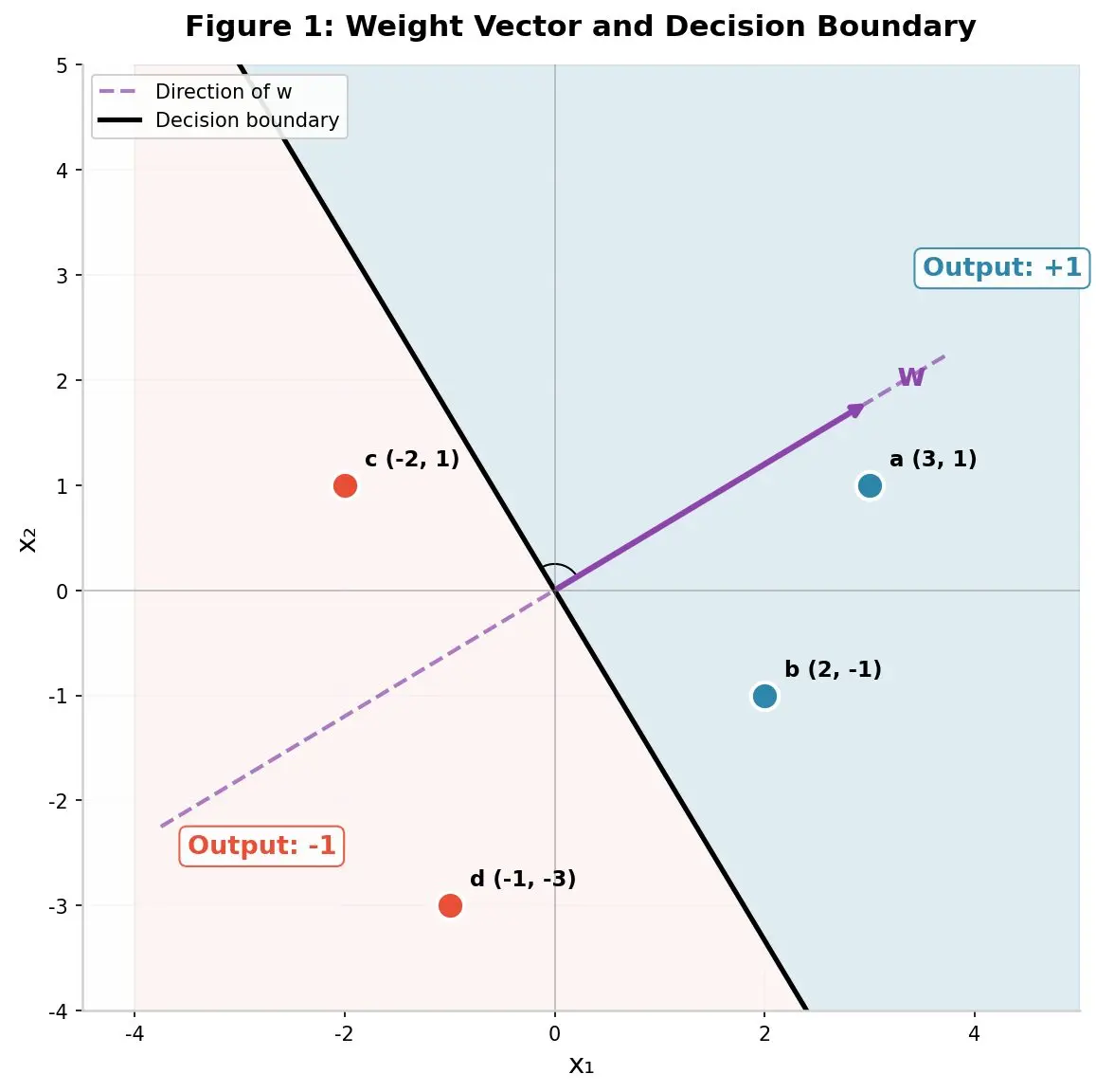
Figure 1: The weight vector w points in a certain direction. The dashed line shows that direction. The solid black line is perpendicular (at 90 degrees) to w. This solid line is the decision boundary — it cuts the plane into two halves.

Here is the key idea: the weight vector w is always perpendicular to the decision line.

The shaded area on one side of the line gives output +1.
The unshaded area on the other side gives output -1.

If you change the weights, the arrow w rotates, and the solid line also rotates to stay perpendicular. If you only change the bias, the line slides left or right like a curtain rod, but its angle stays the same.

So finding the right perceptron is really just finding the right arrow w (and the right bias) so that the line separates your data correctly.

4. The Dot Product — A Simple Test

Now we need a way to check which side of the line a data point lies on. The book introduces a beautiful tool called the dot product.

Do not let the name scare you. The dot product is just:

Multiply the matching numbers.
Add the results.

For example, if:

w = [2.5, 1.5]

a = [3, 1]

Then:

w · a = (2.5 × 3) + (1.5 × 1)

= 7.5 + 1.5

= 9

The dot product is positive. That means point a is on the same side as the arrow w — the shaded side.

Let us check all four points from the book (page 40):

Point	Vector	Dot Product with w	Sign	Side
a	(3, 1)	9.0	+	Shaded (+1)
b	(2, -1)	3.5	+	Shaded (+1)
c	(-2, 1)	-3.5	−	Unshaded (-1)
d	(-1, -3)	-7.0	−	Unshaded (-1)

Look at that! Just by doing simple multiplication and addition, the perceptron knows instantly which group each point belongs to.

If a point lies exactly on the line, the dot product is zero. That point is neither +1 nor -1; it is sitting on the fence.

5. The Bias — Sliding the Line

In the picture above, the line passes through the origin (the center point). But what if the best separating line is somewhere else?

This is where the bias b helps.

Think of the bias as a slide control. It moves the whole line away from the center without tilting it. In the book (page 41), the author shows that if the first attempt misclassifies one point, the perceptron can learn a new bias and shift the line until every point sits on the correct side.

The book also gives an important warning: if the data can be separated by a straight line, there are infinitely many lines that work. The perceptron will find one of them. It does not promise to find the best one. That problem — finding the “best” line — comes later in more advanced methods.

6. Matrices — Numbers in Boxes

So far we have talked about arrows and lines. But computers do not draw arrows. They work with arrays of numbers.

An array with rows and columns is called a matrix. A vector is just a skinny matrix — either one row or one column.

For example:

If you flip a column matrix on its side, you get a row matrix. This flip is called the transpose:

Why is this useful? Because to take the dot product of two column vectors using matrix rules, you transpose one of them:

This looks small, but it is the bridge between pretty geometry and fast computer code. When you see w Tx in a research paper, remember: it is just the dot product we calculated above.

7. Putting It All Together

We started with a long equation full of sums and subscripts. Now we can write the entire perceptron in one tiny, elegant line:

There is one last trick to make it even shorter. Remember the bias b ? We can hide it inside the weight vector by adding a fake input x 0 = 1 and calling the bias w = 0

. Now:

And the equation becomes beautifully simple:

That is it. The weight vector is perpendicular to the separating line. The dot product tells us the side. The sign tells us the answer. Everything in machine learning, from simple perceptrons to giant neural networks, starts from this idea.

8. Python Example: Building a Perceptron from Scratch

Let us bring all of this to life with code. We will build a perceptron using only basic Python — no special machine-learning libraries. We will train it on the same four points from the book: a and b belong to class +1, while c and d belong to class -1.

Here is the complete code:

```

python

class SimplePerceptron:

"""A perceptron built from scratch using only basic Python."""

def __init__(self, n_inputs, learning_rate=0.1):

self.weights = [0.0] * n_inputs

self.bias = 0.0

self.lr = learning_rate

self.history = []

def predict(self, inputs):

activation = self.bias

for i in range(len(inputs)):

activation += self.weights[i] * inputs[i]

return 1 if activation > 0 else -1

def train(self, training_data, labels, epochs=20):

for epoch in range(epochs):

errors = 0

for x, target in zip(training_data, labels):

prediction = self.predict(x)

if prediction != target:

errors += 1

for i in range(len(self.weights)):

self.weights[i] += self.lr * target * x[i]

self.bias += self.lr * target

self.history.append({

'epoch': epoch + 1,

'weights': list(self.weights),

'bias': self.bias,

'errors': errors

})

print(f"Epoch {epoch+1}: weights={self.weights}, bias={self.bias:.3f}, errors={errors}")

if errors == 0:

print(f"Converged at epoch {epoch+1}!")

break

return self.history

# Training data from the book

training_data = [

[3, 1], # a

[2, -1], # b

[-2, 1], # c

[-1, -3] # d

]

labels = [1, 1, -1, -1]

# Train

perceptron = SimplePerceptron(n_inputs=2, learning_rate=0.2)

history = perceptron.train(training_data, labels, epochs=20)

# Test

print("\nPredictions:")

names = ['a', 'b', 'c', 'd']

for name, x, label in zip(names, training_data, labels):

pred = perceptron.predict(x)

status = "Correct" if pred == label else "Wrong"

print(f" {name} {x}: predicted = {pred}, actual = {label} ({status})")

```

In just two epochs, the perceptron found a line that separates all four points perfectly. The learned weights were [0.6,0.2] and the bias was 0.2 .

Notice that this line is different from the book’s example line (which used weights [2.5,1.5] ). That is okay! As the book reminds us, many correct lines exist. The perceptron simply finds the first one that works.

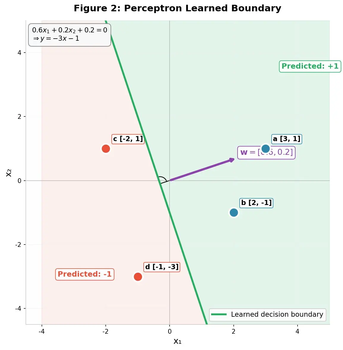
Figure 2: The green line is what our scratch-built perceptron learned. The purple arrow shows the learned weight vector, which is perpendicular to the green line — exactly as the geometry promised.

Reference

Anil Ananthaswamy, Why Machines Learn: The Elegant Math Behind Modern AI (2024),