Probability — The Secret Language of Machine Learning

Machine-Learning tutorial · PySpark.in

​Introduction: Why Should You Care About Probability?

Imagine you are playing a game show. There are three doors. Behind one door is a car, and behind the other two are goats. You pick Door 1. The host, who knows what's behind each door, opens Door 3 and shows you a goat. Then he asks: "Do you want to switch to Door 2?"

What would you do?

Most people say: "It doesn't matter. Now it's 50-50 between Door 1 and Door 2."

But they are wrong! The probability of winning if you switch is 2/3 (66.7%), and if you don't switch, it's only 1/3 (33.3%).

This famous puzzle is called the Monty Hall Problem, and it shows how our human intuition fails when dealing with probability. Machines don't have this problem — they can calculate probabilities perfectly. That's why understanding probability is the foundation of machine learning.

In this blog, we will learn all the probability concepts from Chapter 4 of Anil's book, step by step, in the simplest way possible.

​Part 1: The Monty Hall Problem — Probability is Tricky!

Let's understand why switching gives you better odds.

​The Setup:

• 3 doors: Car behind one, goats behind two
• You pick Door 1
• Host opens Door 3 (goat)
• Should you switch to Door 2?

​The Key Insight:

Think of it this way: When you first picked Door 1, you had a 1/3 chance of being right. That means there was a 2/3 chance the car was behind Door 2 or Door 3 combined.

When the host opens Door 3 (showing a goat), that 2/3 probability now concentrates entirely on Door 2!

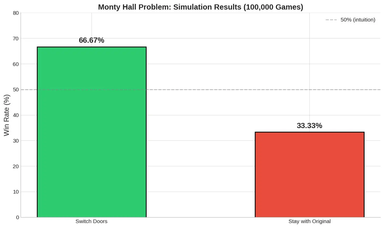
Figure: Simulation showing probability of winning — switching wins ~67% of the time, not switching wins ~33%

Anil shares a fascinating story in his book: Even the great mathematician Paul Erdős refused to believe you should switch! It took a computer simulation of 100,000 games to convince him. This shows that probability is powerful but often counterintuitive.

​Part 2: Bayes's Theorem — Updating Your Beliefs

​The Disease Test Example

Imagine a disease that affects 1 in 1,000 people (0.1%). There's a test that is 90% accurate:

• If you have the disease, it says "positive" 90% of the time
• If you don't have the disease, it says "negative" 90% of the time

You take the test. It says POSITIVE. What's the chance you actually have the disease?

Most people say: "90%!"

But the correct answer is only about 0.89% — less than 1%!

​How? Using Bayes's Theorem

Thomas Bayes gave us a formula to update our beliefs when we get new evidence:

P(H | E) = [ P(H) × P(E | H) ] / P(E)

​

Where:

• P(H) = Prior probability (belief before evidence) = 0.001 (1 in 1000)
• P(E|H) = Likelihood (probability of positive test IF you have disease) = 0.9
• P(E) = Total probability of positive test = (0.001 × 0.9) + (0.999 × 0.1) = 0.1008

P(H | E) = (0.001 × 0.9) / 0.1008

​

=0.0089≈0.89%

Why so low? Because the disease is rare! Most positive tests are false positives from healthy people.

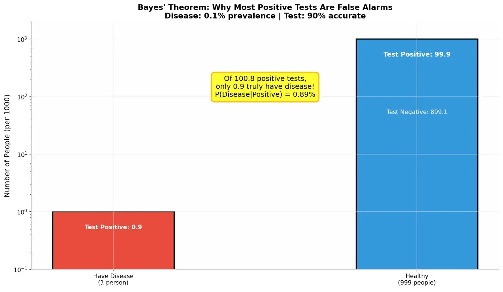
Figure: Even with a good test, rare diseases mean most positives are false alarms

​Bayes's Theorem in Simple Words:

"Your new belief = (Your old belief × How likely the evidence is if your belief is true) ÷ How likely the evidence is overall"

​Part 3: Random Variables — Giving Numbers to Outcomes

A random variable is just a way to assign numbers to outcomes of an experiment.

​Two Types of Random Variables:

1. Discrete Random Variable: Takes specific, separate values

• Coin toss: only 0 or 1
• Dice roll: only 1, 2, 3, 4, 5, or 6

2. Continuous Random Variable: Can take any value in a range

• Temperature: 98.6°F, 98.61°F, 98.612°F... infinite possibilities
• Height, weight, time

​Part 4: Probability Distributions — The Shape of Chance

​Discrete: Probability Mass Function (PMF)

For discrete variables, we use a Probability Mass Function. It tells us the probability of each specific value.

Example: Fair Coin

P(X=0)=0.5,P(X=1)=0.5

Example: Biased Coin (p = 0.6 for heads)

P(X = x) = {

1 - p if x = 0

p if x = 1

}

​

This is called the Bernoulli Distribution — the simplest probability distribution.

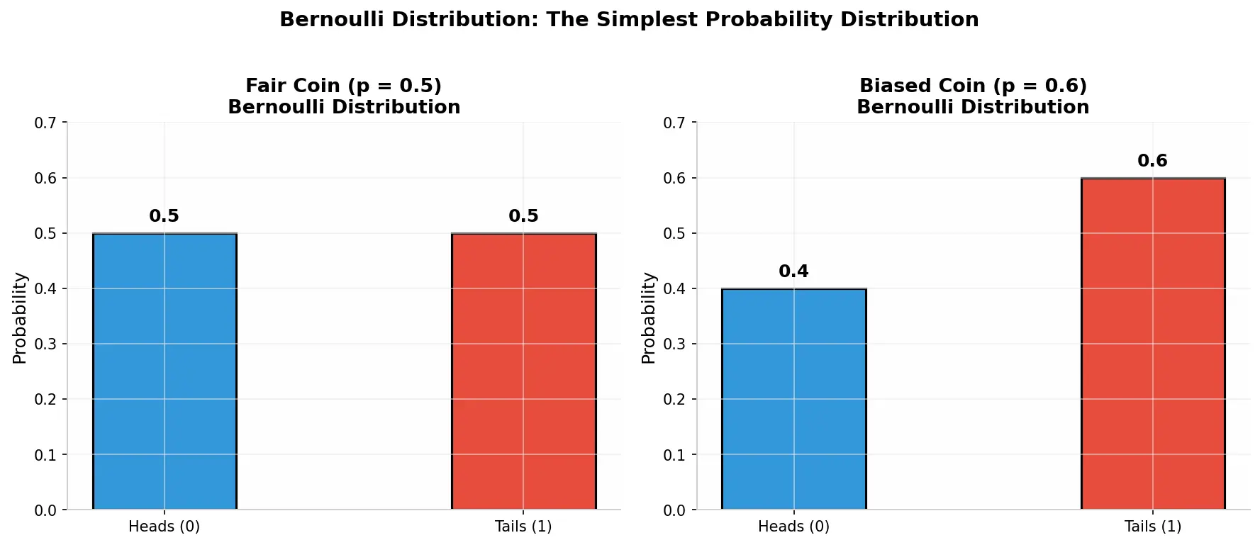
Figure: Bernoulli distribution for fair coin (p=0.5) and biased coin (p=0.6)

​Continuous: Probability Density Function (PDF)

For continuous variables, we can't ask "What's the probability of exactly 98.6°F?" because the answer is zero (there are infinite possible values)!

Instead, we ask: "What's the probability the temperature is between 98.5°F and 98.7°F?"

This probability equals the area under the curve between those points.

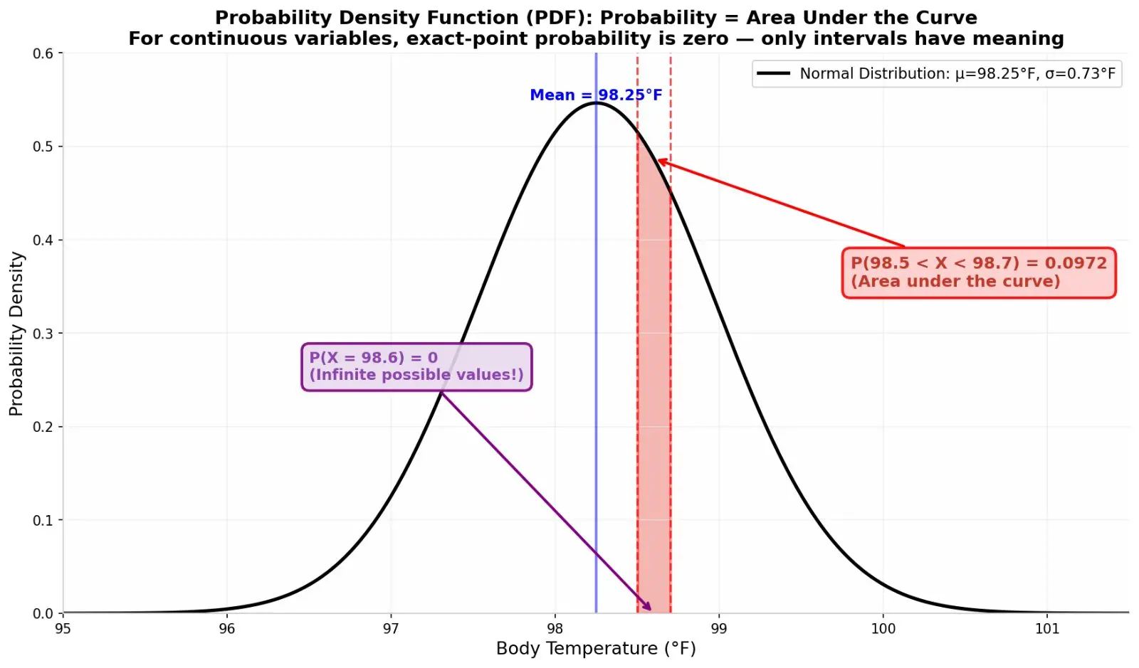
Figure: Normal distribution for body temperature. The area between two values gives the probability

​Part 5: The Normal (Gaussian) Distribution — Nature's Favorite Curve

The normal distribution looks like a bell. It's everywhere in nature:

• Heights of people
• Test scores
• Measurement errors
• Blood pressure readings

​Key Properties:

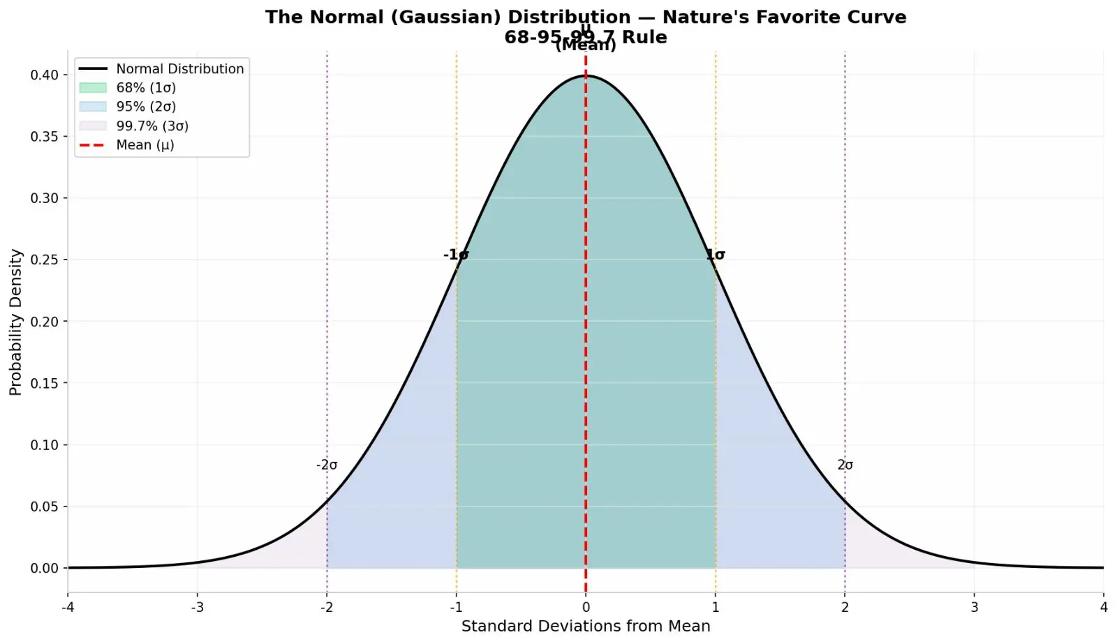
Figure: Normal distribution showing mean and standard deviation regions

The 68-95-99.7 Rule:

• 68% of data falls within 1 standard deviation of mean
• 95% within 2 standard deviations
• 99.7% within 3 standard deviations

Example: If average body temperature is 98.25°F with standard deviation 0.73°F:

• 68% of people have temperature between 97.52°F and 98.98°F
• Almost everyone (99.7%) is between 96.06°F and 100.44°F

​Part 6: Expected Value, Variance, and Standard Deviation

​Expected Value (E[X]) — The "Average" You'd Expect

For a discrete random variable:

E(X) = (k = 1nx) n

Example: A rigged digital display shows numbers 0-6 with these probabilities:

E(X) = 0×(1/32) + 1×(1/16) + 2×(1/8) + 3×(9/16) + 4×(1/8) + 5×(1/16) + 6×(1/32)

E(X) = 0 + 0.0625 + 0.25 + 1.6875 + 0.5 + 0.3125 + 0.1875 = 3.0

The expected value is 3 — which makes sense because 3 has the highest probability (9/16).

​Variance — How Spread Out Things Are

Var(X) = k = 1n(xk - E(X)) 2xP (X = xk)

Variance measures: "On average, how far are values from the mean?"

​Standard Deviation

sd = sqrt(Var(X)) = sigma

Standard deviation is just the square root of variance. It's in the same units as your original data, making it easier to understand.

​Part 7: Sampling — Learning from Data

​Theoretical vs. Empirical Probability

The Law of Large Numbers: As you do more experiments, your empirical probability gets closer to the true theoretical probability.

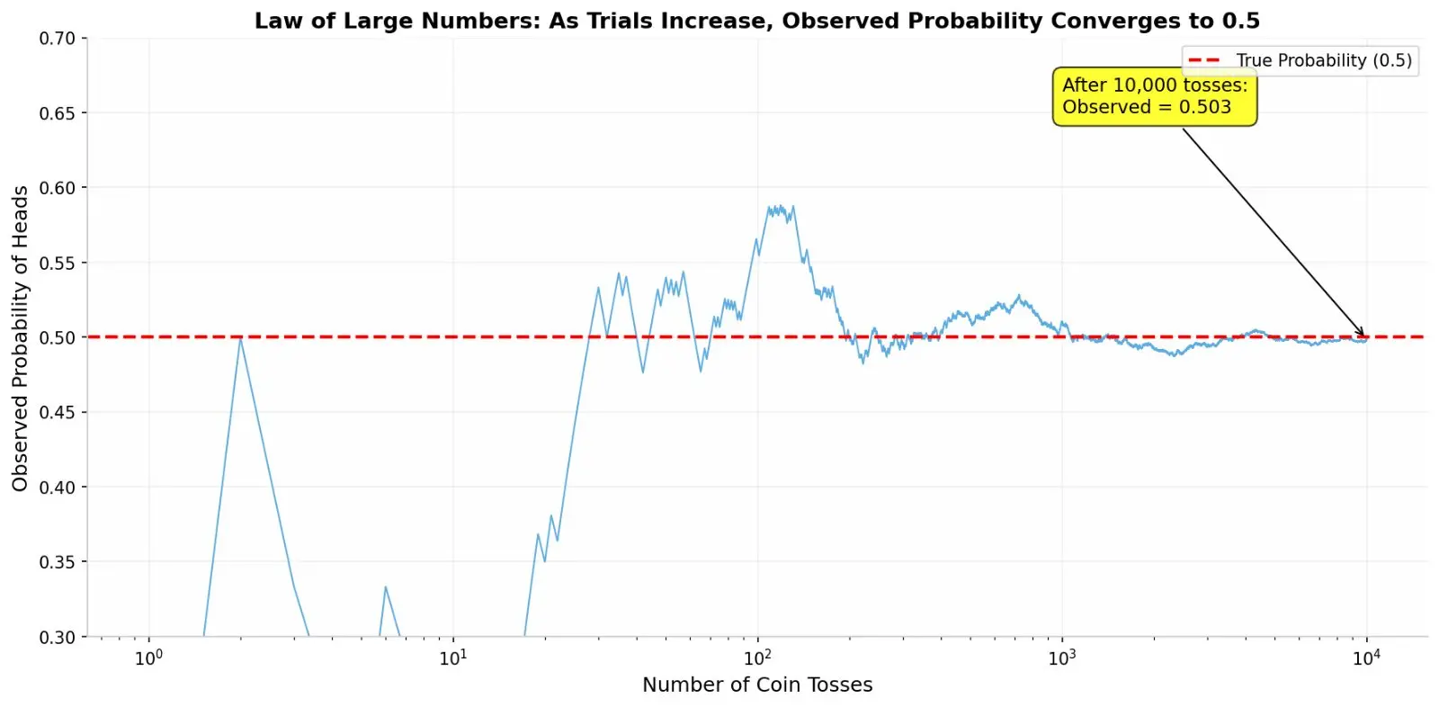
Figure: As number of coin tosses increases, observed probability converges to 0.5

​Part 8: Supervised Learning — The Probability View

Now we connect probability to machine learning!

​The Setup:

You have data about people:

• X = features (height, weight, cholesterol, blood pressure, etc.)
• y = label (1 = had heart attack in 5 years, -1 = did not)

Each row of data is a d-dimensional vector: [x₁, x₂, x₃, ..., xₙ]

​The Goal:

Learn a function f(x) that predicts y:

f(x)=y

But we can also think probabilistically: Learn the underlying probability distribution P(X, y).

If we knew this distribution perfectly, we could calculate:

• P(y = at-risk | x) = probability person is at risk given their features
• P(y = not-at-risk | x) = probability person is not at risk

Then predict the class with higher probability. This perfect classifier is called the Bayes Optimal Classifier.

Important Reality Check: We almost never know the true underlying distribution! ML algorithms try to estimate it from limited data. That's why:

• All ML algorithms make mistakes
• 100% accuracy is impossible
• More data usually helps (but not always!)

​Part 9: Estimating Distributions — MLE and MAP

Since we don't know the true distribution, how do we estimate it?

​Method 1: Maximum Likelihood Estimation (MLE)

Idea: Find the parameters θ that make your observed data most likely.

Steps:

1. Assume a distribution type (Bernoulli, Normal, etc.)
2. Write the likelihood function P(Data | θ)
3. Find θ that maximizes this likelihood

Example: You have heights of "tall" and "short" people. Assume each group follows a normal distribution. MLE finds the mean and standard deviation that best fit your data.

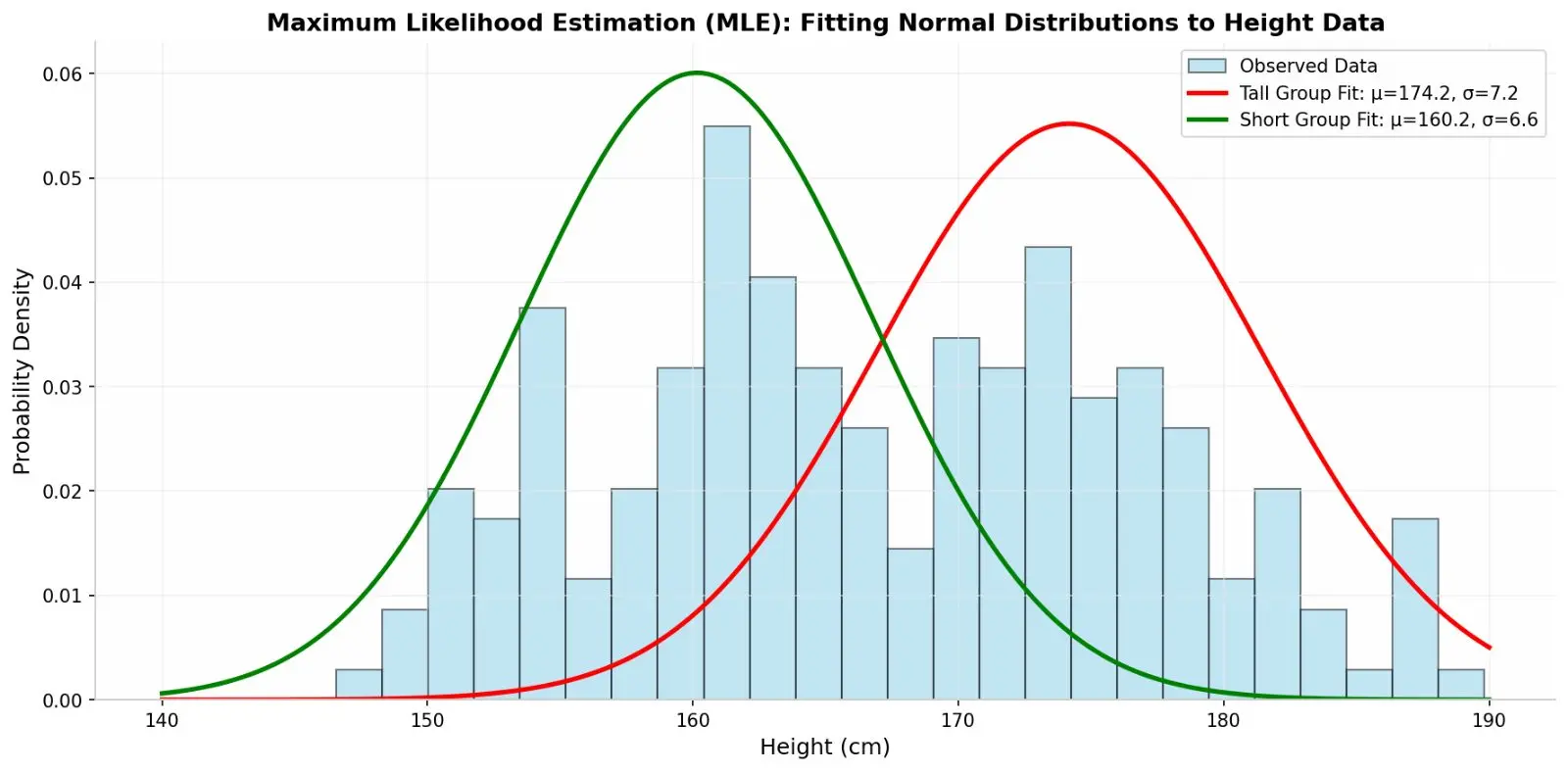
Figure: Fitting a normal distribution to observed height data using MLE

​Method 2: Maximum A Posteriori (MAP)

Idea: Same as MLE, but start with a prior belief about θ.

This is the Bayesian approach:

1. Start with prior: P(θ) — your belief before seeing data
2. See data
3. Update to posterior: P(θ | Data) using Bayes's theorem

P(theta | Data) = (P(Data | theta)xP(theta))/(P(Data))

​

MLE vs MAP:

• MLE works best with lots of data
• MAP works better with less data (prior helps when data is scarce)
• As data grows, MAP and MLE give similar answers

​The Basic Algorithm (for both):

1. Write the function to maximize

2. Take derivative with respect to θ

3. Set derivative = 0 (find the peak)

4. Solve for θ

5. If no closed-form solution: use gradient descent

​Part 10: The Federalist Papers — Real-World Bayesian Analysis

Anil shares a fascinating historical example. In 1787-88, 85 essays called "The Federalist Papers" were published anonymously under the name "Publius." Historians knew:

• Alexander Hamilton wrote some
• James Madison wrote some
• John Jay wrote some
• 12 papers were disputed: Hamilton or Madison?

In 1941, statisticians Frederick Mosteller and David Wallace used Bayesian analysis to solve this!

​Their Approach:

1. Look at function words (prepositions, conjunctions, articles): "upon," "by," "to," "from"
2. Count how often each author used these words
3. Use Bayes's theorem to calculate probability of authorship

Key Insight: The more separated the word-usage distributions of two authors, the better that word discriminates between them.

Result: Overwhelming evidence that Madison wrote the disputed papers!

This was one of the first large-scale uses of Bayesian reasoning in machine learning.

​Part 11: Penguins! — A Complete ML Example

Now let's put everything together with a concrete example from Anil's book.

​The Data:

Kristen Gorman collected data on 334 penguins from Antarctica:

• 3 species: Adélie, Gentoo, Chinstrap
• 5 features per penguin: bill length, bill depth, flipper length, body mass, sex

Each penguin is a point in 5-dimensional space: [x₁, x₂, x₃, x₄, x₅]

​The Problem:

Given a penguin's features, predict its species.

​Visualization — Why This Matters:

2D Plot: Bill Length vs Bill Depth

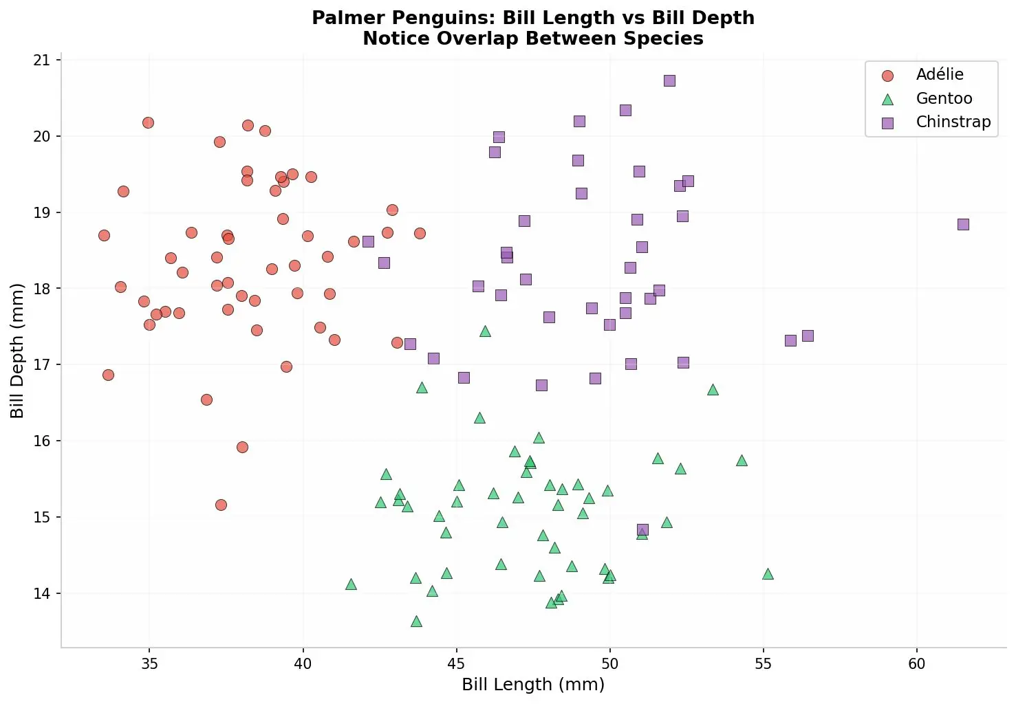
Figure: Adélie (circles) and Gentoo (triangles) show some separation, but there's overlap

3D Plot: Adding Another Feature

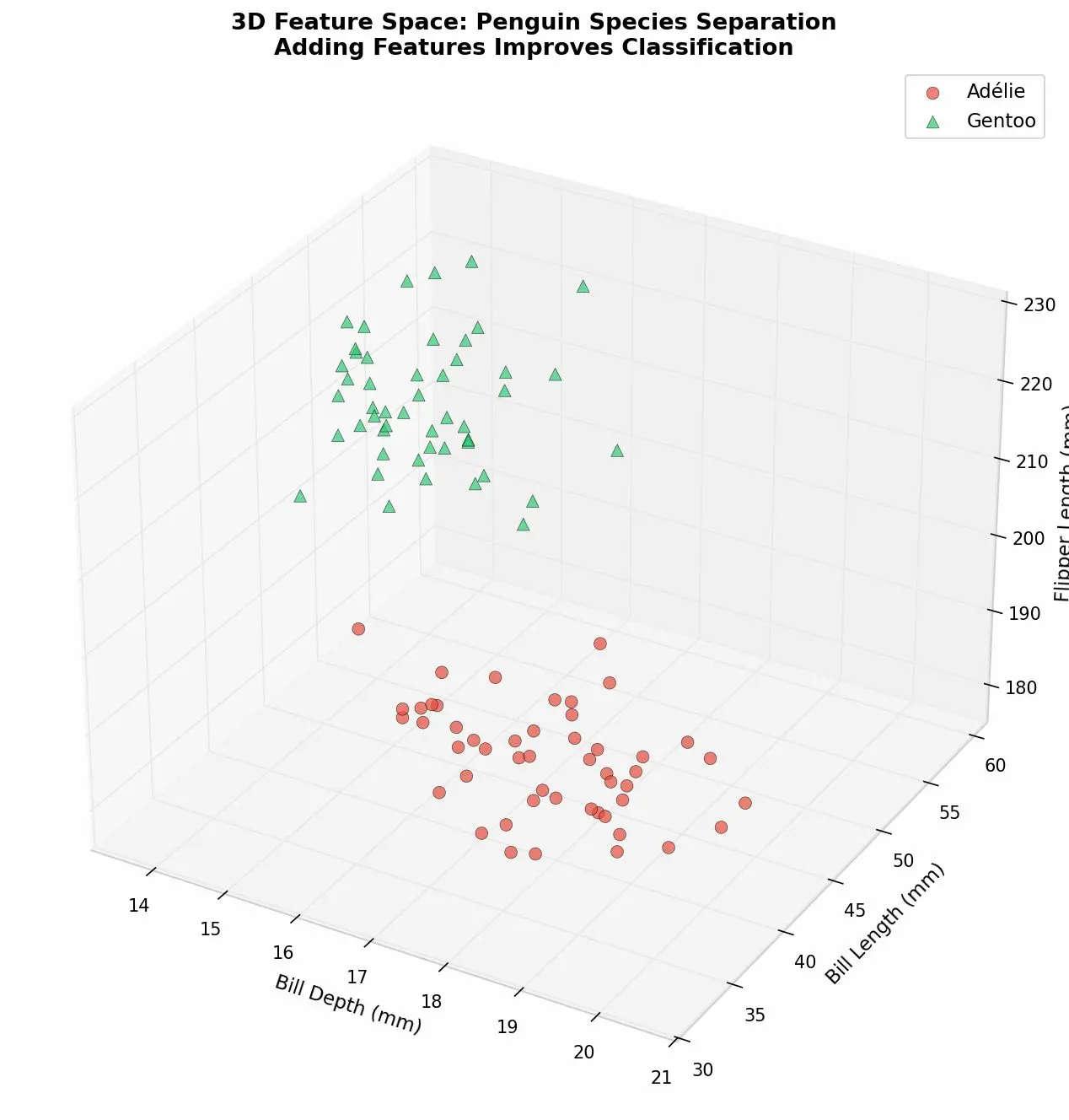
Figure: Probability density surfaces for two penguin species in 3D feature space

All Three Species:

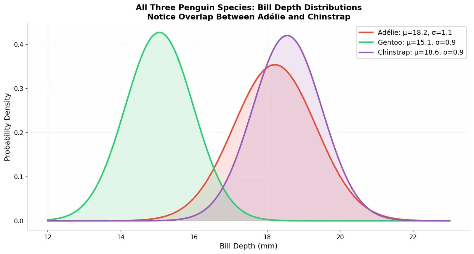
Figure: All three species plotted together — notice the overlap between Adélie and Chinstrap

​The Challenge:

With more features, we need to estimate higher-dimensional distributions. This becomes very hard with limited data!

​Part 12: Building a Bayes Optimal Classifier

​Step 1: Look at One Feature (Bill Depth)

Adélie Penguins — Histogram:

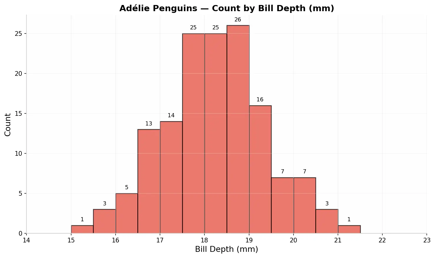
Figure: Count of Adélie penguins by bill depth (mm)

We can fit a normal distribution to this data:

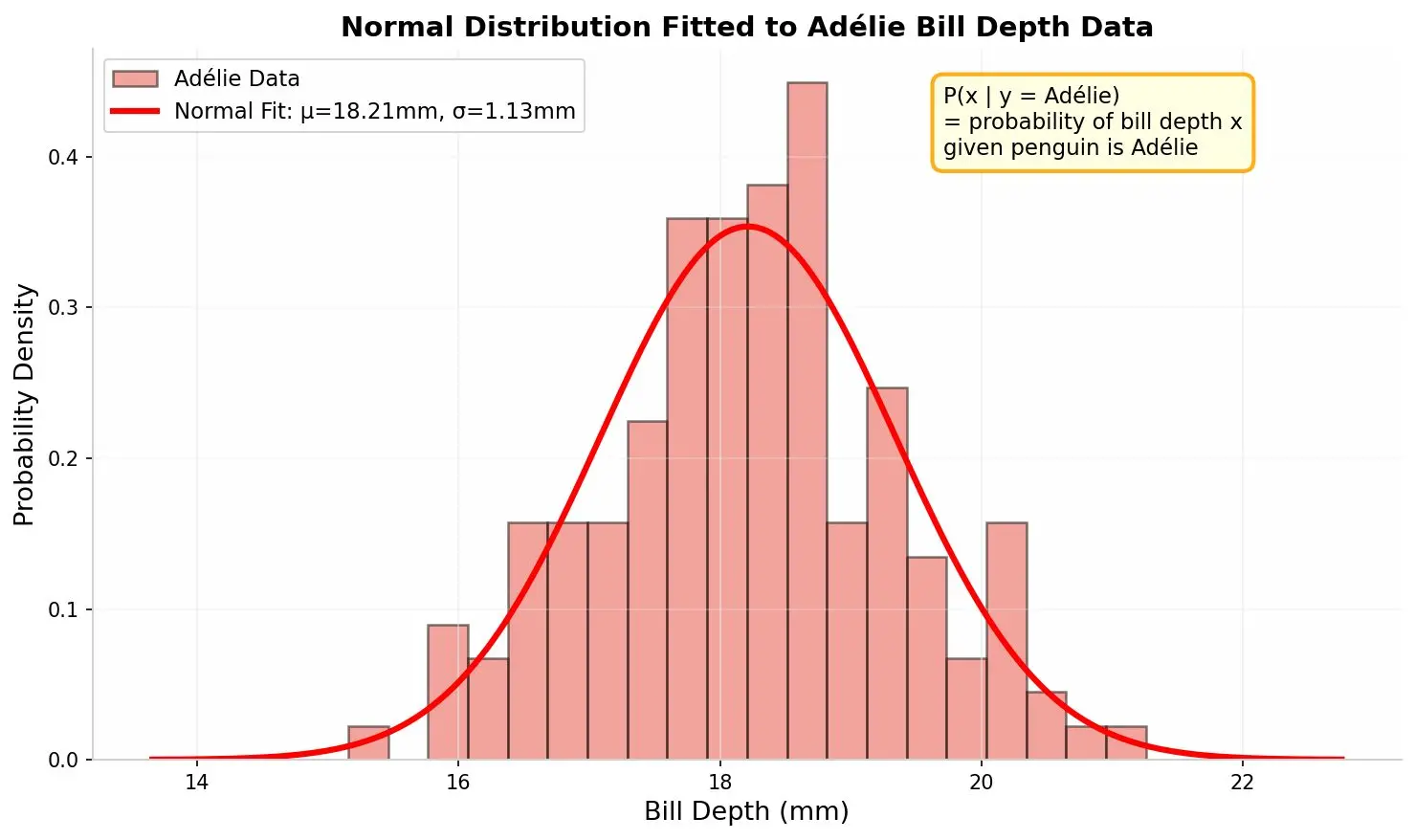
Figure: Normal distribution fitted to Adélie bill depth data

This gives us: P(x | y = Adélie) = probability of bill depth x given that penguin is Adélie

Gentoo Penguins — Same Process:

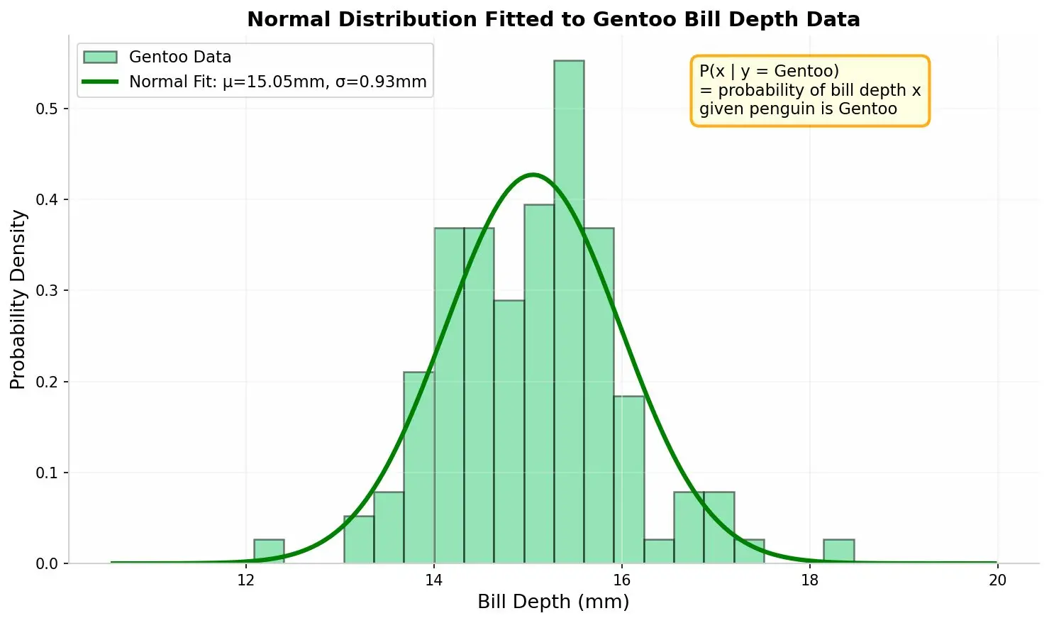
Figure: Normal distribution fitted to Gentoo bill depth data

​Step 2: Apply Bayes's Theorem

We want: P(y = species | x) = probability of species given bill depth

Using Bayes's theorem:

P(y = Gentoo | x) = (P(x | y = Gentoo)xP(y = Gentoo))/(P(x))

P(y = Adeˊlie | x) = (P(x | y = Adeˊlie)xP(y = Adeˊlie))/(P(x))

​

Where:

• P(y = Gentoo) = prior = 119/(119+146) = 0.45 (from training data)
• P(y = Adélie) = prior = 146/(119+146) = 0.55
• P(x | y) = read from our fitted normal curves
• P(x) = same for both, so we can ignore it when comparing!

​Step 3: Make Prediction

For a new penguin with bill depth = 16 mm:

• Calculate P(Gentoo | 16) and P(Adélie | 16)
• Predict the species with higher probability

Example Calculation:

• P(Gentoo | 16) might be 0.8
• P(Adélie | 16) might be 0.2
• Predict: Gentoo (but there's 20% chance we're wrong!)

Even the Bayes Optimal Classifier makes errors — that's the irreducible error set by nature.

​When One Feature Isn't Enough:

Bill depth alone cannot distinguish Adélie from Chinstrap — their distributions overlap too much!

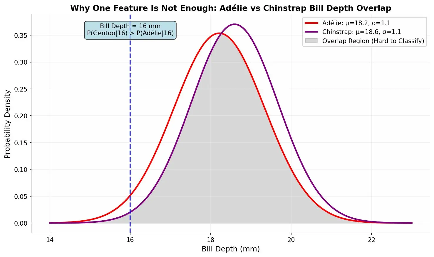
Figure: Adélie and Chinstrap bill depth distributions overlap significantly

Solution: Use more features (bill length AND bill depth together)!

​Part 13: The Curse of Dimensionality — Why More Features Can Hurt

Adding features seems good, but there's a problem:

The problem: To estimate a distribution accurately in high dimensions, you need exponentially more data. With limited samples, the task becomes nearly impossible.

​Part 14: Naïve Bayes — A Clever Simplification

​The Problem:

We need to estimate P(x₁, x₂, x₃, x₄, x₅ | y) — the joint probability of all five features given species.

This is a complicated surface in 6 dimensions. With limited data, we can't estimate it well.

​The "Naïve" Trick:

Assume all features are independent of each other!

This means:

• Bill depth variation has nothing to do with bill length variation
• Each feature is sampled from its own separate distribution

This is NEVER really true in nature! But it makes the math much easier.

​The Math Becomes Simple:

Instead of one big complicated probability:

P(x | y = A) = P(x 1 ,x 2 ,x 3 ,x 4 ,x 5 | y = A)

P(x | y = A) = P(x 1 | y = A)xP(x 2 | y = A)xP(x 3 | y = A)xP(x 4 | y = A)xP(x 5 | y = A)

P(x | y = A) = i = 15P(x i | y = A)

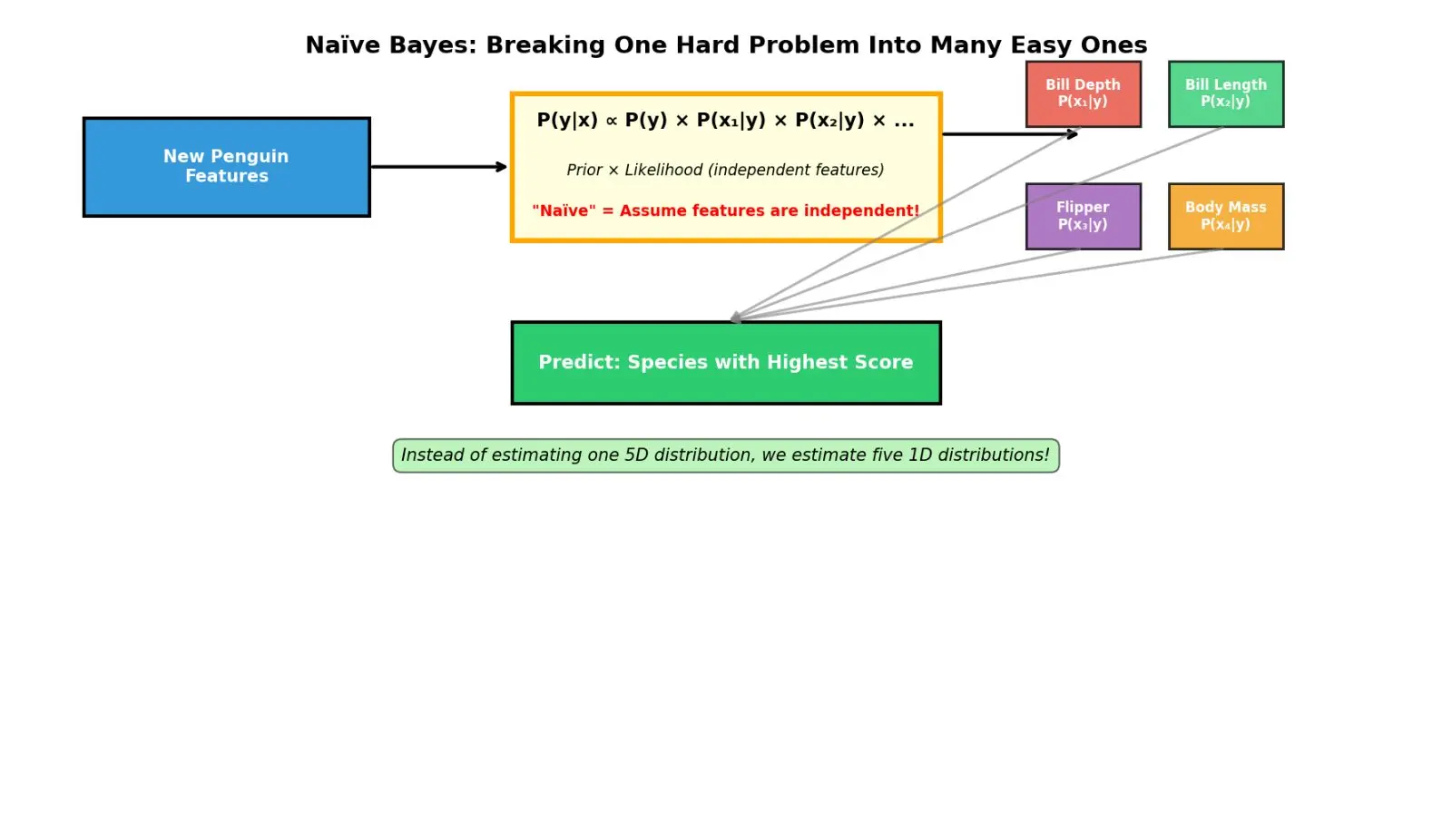
Figure: Naïve Bayes breaks one hard problem into many easy problems

​Why This Works:

• We only need to estimate one-dimensional distributions
• Needs much less data
• Computationally far less intensive
• Surprisingly accurate in practice!

This classifier is called Naïve Bayes (or jokingly, "Idiot Bayes"). It's used for:

• Spam detection
• Sentiment analysis
• Medical diagnosis
• And many more applications!

​Part 15: Generative vs. Discriminative Learning

Two major approaches to ML:

​Generative Learning:

• Learn the full joint distribution P(X, y)
• Can generate new data that looks like training data
• Example: Naïve Bayes
• This is the foundation of Generative AI!

​Discriminative Learning:

• Learn P(y | x) directly — just the boundary between classes
• Don't care about the full distribution
• Examples: Perceptron, Neural Networks, SVM
• Often works better for pure prediction

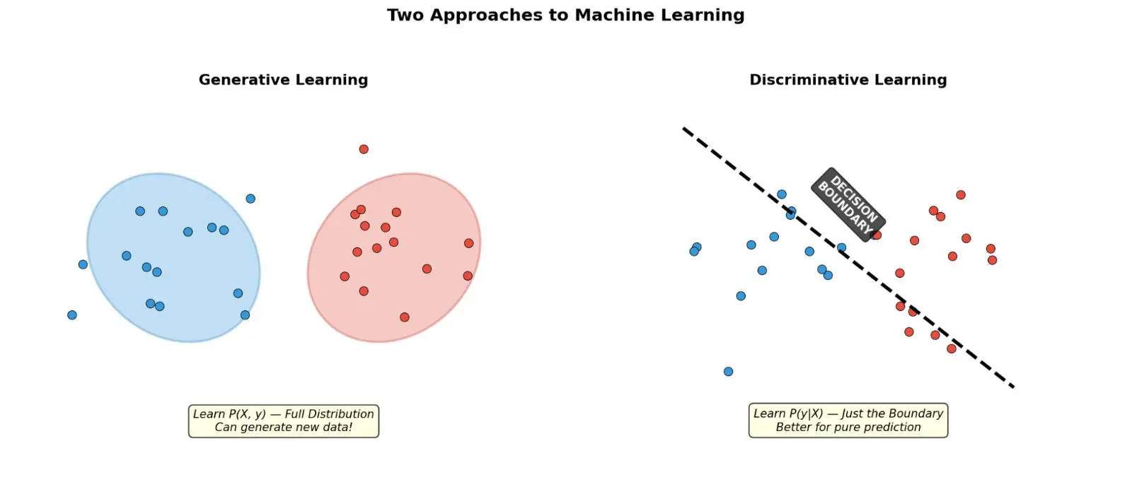
Figure: Generative models learn the full distribution; discriminative models learn just the decision boundary

​Part 16: Wrap-Up — Key Takeaways

​What We Learned in This Chapter:

​Python Implementation: Naïve Bayes from Scratch

Let's implement a simple Gaussian Naïve Bayes classifier without any libraries!

```

"""

Gaussian Naive Bayes from Scratch

=================================

Without using classes

"""

import math

# Store model information globally

classes = []

parameters = {}

priors = {}

def mean(numbers):

"""Calculate mean."""

return sum(numbers) / len(numbers)

def std_dev(numbers):

"""Calculate standard deviation."""

avg = mean(numbers)

variance = sum((x - avg) ** 2 for x in numbers) / len(numbers)

return math.sqrt(variance)

def gaussian_pdf(x, mean_value, std):

"""

Probability Density Function for Gaussian distribution

"""

if std == 0:

return 1.0 if x == mean_value else 0.0

exponent = math.exp(

-0.5 * ((x - mean_value) / std) ** 2

)

return (

1 /

(std * math.sqrt(2 * math.pi))

) * exponent

def fit(X, y):

"""

Train model

"""

global classes, parameters, priors

classes = list(set(y))

data_by_class = {c: [] for c in classes}

# Separate data by class

for features, label in zip(X, y):

data_by_class[label].append(features)

# Calculate prior and statistics

for c in classes:

priors[c] = len(data_by_class[c]) / len(X)

num_features = len(X[0])

parameters[c] = []

for feature_idx in range(num_features):

feature_values = [

sample[feature_idx]

for sample in data_by_class[c]

]

avg = mean(feature_values)

std = std_dev(feature_values)

parameters[c].append(

(avg, std)

)

def predict_single(x):

"""

Predict one sample

"""

best_class = None

best_score = float("-inf")

for c in classes:

score = math.log(priors[c])

for feature_idx, value in enumerate(x):

avg, std = parameters[c][feature_idx]

pdf = gaussian_pdf(

value,

avg,

std

)

if pdf > 0:

score += math.log(pdf)

else:

score += math.log(1e-300)

if score > best_score:

best_score = score

best_class = c

return best_class

def predict(X):

"""

Predict multiple samples

"""

return [

predict_single(x)

for x in X

]

# ====================================

# DEMO

# ====================================

training_data = [

# Adelie

([18.0, 38.0], "Adelie"),

([17.5, 39.0], "Adelie"),

([19.0, 37.0], "Adelie"),

([18.5, 38.5], "Adelie"),

([17.0, 39.5], "Adelie"),

([18.0, 38.5], "Adelie"),

# Gentoo

([15.0, 45.0], "Gentoo"),

([14.5, 46.0], "Gentoo"),

([15.5, 44.5], "Gentoo"),

([14.0, 47.0], "Gentoo"),

([15.0, 46.0], "Gentoo"),

([14.5, 45.5], "Gentoo"),

]

X_train = [

x for x, y in training_data

]

y_train = [

y for x, y in training_data

]

# Train model

fit(X_train, y_train)

print("=" * 50)

print("NAIVE BAYES FROM SCRATCH")

print("=" * 50)

print("\nLearned Parameters:")

for c in classes:

print(f"\nClass: {c}")

print(

f"Prior: {priors[c]:.3f}"

)

for i, (avg, std) in enumerate(parameters[c]):

feature_name = [

"Bill Depth",

"Bill Length"

][i]

print(

f"{feature_name}: "

f"mean={avg:.2f}, "

f"std={std:.2f}"

)

test_samples = [

[18.0, 38.0],

[15.0, 45.0],

[17.5, 39.0],

[14.5, 46.5]

]

print("\nPredictions:")

for sample in test_samples:

result = predict_single(sample)

print(

f"{sample} -> {result}"

)

```

​Output of the Program:

​Key Points from the Code:

1. No external libraries — pure Python math
2. Gaussian PDF implements the bell curve formula
3. Log probabilities prevent numerical underflow when multiplying many small numbers
4. Naïve assumption means we multiply individual feature probabilities
5. Bayes' theorem in action: prior × likelihood for each class

​Conclusion

Probability is the language of uncertainty, and machine learning is all about handling uncertainty. From the counterintuitive Monty Hall problem to the practical Naïve Bayes classifier, we've seen how probability theory gives ML algorithms their power.

Remember:

• Perfect prediction is impossible — even the Bayes Optimal classifier makes errors
• More data helps, but dimensionality can hurt
• Simplifying assumptions (like independence in Naïve Bayes) often work surprisingly well
• The goal is not perfection, but doing the best we can with available information

​Reference

Why Machines Learn: The Elegant Math Behind Modern AI" by Anil Ananthaswamy (2024).

More Machine-Learning tutorials

• Introduction to Machine Learning
• Introduction to Deep Learning
• ​A Beginner's Guide to Machine Learning
• The First Artificial Neuron and Learning from Mistakes
• ​Patterns
• ​ Understanding Vectors, the Building Blocks of AI

All tutorials · Try the free PySpark compiler · Practice challenges