Gradient Descent
Machine-Learning tutorial · PySpark.in
1. Introduction: Lost on a Hillside
Imagine you are standing on a rice terrace high up on a hillside in Vietnam. It is getting dark. Down in the valley, you can see the lights of a village — your destination. But you can only see a few feet ahead of you. The hillside is steep, but not too steep to walk down. How do you get to the village?
You cannot see the entire path. You cannot plan a straight line from where you are to where you want to be. So what do you do?
You stand at the edge of your terrace. You look around. You find the steepest way down to the next terrace below. You walk along that terrace until you find the next steepest drop. You repeat this again and again — terrace by terrace, step by step — until you finally reach the village.
This is not just a story about hiking. This is exactly how the most important algorithm in machine learning works. It is called Gradient Descent, and it is the reason why machines can learn.
In this blog, we will follow Chapter 3 of Why Machines Learn — from the rice terraces of Vietnam to the mathematical "bottom of the bowl," and finally to a legendary weekend at Stanford in 1959 when two scientists named Widrow and Hoff invented an algorithm that became the foundation of all modern AI.
By the end of this blog, you will understand:
- Why walking down a hill is the same as teaching a machine
- What a "gradient" really means (in simple words)
- Why some hills are easy to descend and others are dangerous traps
- How two men on a blackboard created the algorithm that powers every neural network today
2. The Rice Terrace Analogy: Learning by Feeling the Slope
The book opens Chapter 3 with this beautiful image: rice paddies carved into hillsides in China, Japan, and Vietnam. Each terrace is flat. The edges are steep. If you want to go down, you cannot just run straight — you would fall off the cliff! Instead, you walk along the flat terrace until you find the safest, steepest drop to the next level.
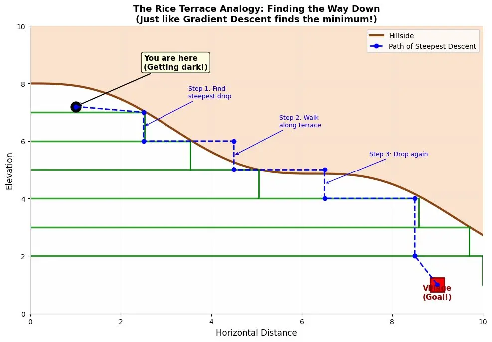
The picture above shows the analogy. You start at the top (dark, scary, lost). The green horizontal lines are the terraces. The blue dashed line with circles shows your path: you walk along a terrace, find the steepest drop, descend, walk along the next terrace, find the next drop, and so on — until you reach the village at the bottom.
This is the method of steepest descent. In everyday language, it means: at every step, move in the direction that decreases your height the fastest.
But here is the key insight: you do not need to see the whole mountain. You only need to know which way is down from where you are standing right now. That local information — the slope at your current position — is enough to guide you to the bottom.
This is exactly what machines do when they "learn." They do not know the perfect answer from the start. But they can measure whether they are getting better or worse. They take small steps in the direction that makes them better. And if they keep doing this, they eventually reach the best possible answer.
3. The Bottom of the Bowl: Understanding Gradients with a Simple Curve
Now let us make this mathematical — but still very simple. The book introduces the curve y = x². You have probably seen this before. It looks like a bowl that opens upward.
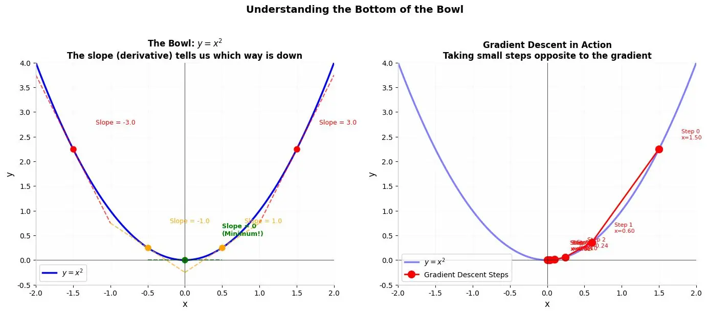
On the left, the blue curve is y = x² — a simple bowl. The colored dots show different points, and the dashed lines show the tangent (the "slope") at each point. At x = 1.5, the slope is 3 (steep). At x = 0.5, the slope is 1 (gentle). At x = 0, the slope is 0 — this is the bottom of the bowl!
What is a Slope?
The slope tells you how steep the curve is at a particular point. Think of it like this:
- If the slope is positive, the curve is going up as you move right.
- If the slope is negative, the curve is going down as you move right.
- If the slope is zero, you are at the top or bottom — a flat point.
For the curve y = x², the slope at any point x is given by 2x. This comes from calculus, but the book gives it to us directly. Let us check:
- At x = 2, slope = 2 × 2 = 4 (very steep upward)
- At x = 1, slope = 2 × 1 = 2 (moderately steep upward)
- At x = 0, slope = 2 × 0 = 0 (flat — this is the minimum!)
- At x = -1, slope = 2 × (-1) = -2 (steep downward)
The Derivative: A Fancy Word for "Slope"
The book introduces the word derivative. Do not be scared! As the book quotes from Silvanus P. Thompson's classic Calculus Made Easy (1910): the symbol d simply means "a little bit of." So dy/dx is "a little bit of y divided by a little bit of x" — in other words, the slope.
For y = x², the derivative is dy/dx = 2x. This tells us the slope at every point on the curve.
Gradient Descent: Walking Down the Bowl
Now here is the magic formula for gradient descent:

Where:
- η (eta) is the step size — how big a step you take
- gradient is the slope at your current position (2x for our bowl)
Let us say we start at x = 1.5 and use η = 0.3:
- Step 1: gradient = 2 × 1.5 = 3. New x = 1.5 − 0.3 × 3 = 0.6
- Step 2: gradient = 2 × 0.6 = 1.2. New x = 0.6 − 0.3 × 1.2 = 0.24
- Step 3: gradient = 2 × 0.24 = 0.48. New x = 0.24 − 0.3 × 0.48 = 0.096
See what is happening? x is getting closer and closer to 0 — the bottom of the bowl! And the steps are getting smaller and smaller because the gradient is shrinking.
The right side of the figure above shows this in action. The red dots trace the path of gradient descent, starting from x = 1.5 and zigzagging down to the bottom. Each step is labeled so you can follow the journey.
Why Step Size Matters
The book emphasizes that the step size η must be small. Why?
Imagine you are near the bottom of the bowl but you take a giant step. You might overshoot and end up on the other side of the bowl — higher than where you started! Then your next step might overshoot again, and you could bounce back and forth forever, never settling at the bottom.
With a small step size, you approach the bottom carefully. As the gradient gets smaller near the bottom, your steps automatically get smaller too. It is like walking down a staircase where the steps shrink as you near the ground floor.
4. The 3D Bowl: When There Are Two (or More) Directions
So far, we have only looked at curves with one variable (x). But real machine learning problems have many variables. The book now introduces the 3D bowl: z = x² + y².
This is called an elliptic paraboloid. It looks like a bowl in three dimensions. If you stand anywhere on this surface and look around, you can move in two directions: along the x-axis and along the y-axis.
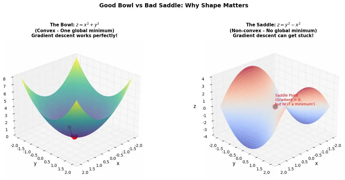
The left image shows the 3D bowl z = x² + y². It is convex — it has one clear bottom. The red dots show gradient descent happily walking down to the minimum. The right image shows a dangerous surface called a saddle (z = y² − x²). It looks like a horse saddle. The center point has gradient zero, but it is NOT a minimum — it is a trap!
Partial Derivatives: Slopes in Each Direction
When we have multiple variables, we need to know the slope in each direction separately. These are called partial derivatives.
For z = x² + y²:
- The partial derivative with respect to x is ∂z/∂x = 2x (treat y as constant)
- The partial derivative with respect to y is ∂z/∂y = 2y (treat x as constant)
Together, these form a vector called the gradient:
∇z = [2x, 2y]
This vector points in the direction of steepest ascent — the fastest way UP. To go down, we move in the opposite direction: −∇z.
An Example: Standing at (3, 4)
The book gives a concrete example. Suppose you are standing at the point where x = 3 and y = 4 on the bowl. The height is z = 3² + 4² = 25.
The gradient at this point is:
- ∂z/∂x = 2 × 3 = 6
- ∂z/∂y = 2 × 4 = 8
So the gradient vector is [6, 8]. This is an arrow pointing from the origin to the point (6, 8). It tells you: "The steepest way up is in this direction." Therefore, to go down, you walk in the opposite direction: −[6, 8] = [−6, −8].
The book beautifully notes: "If you write these numbers in this form, it looks like something very familiar: [6, 8]. It's a vector!" This is the power of calculus — it gives us a compass arrow that tells us which way to walk.
The Dangerous Saddle: When Gradient Descent Fails
Not all surfaces are friendly bowls. The book introduces the hyperbolic paraboloid: z = y² − x². This looks like a horse saddle.
At the point (0, 0), the gradient is zero. But this is NOT the bottom! It is a saddle point — an unstable place. If you move along the y-direction, you go up (like the front and back of a saddle). If you move along the x-direction, you go down (like the sides of a saddle).
If gradient descent lands exactly on a saddle point, it gets confused. The gradient is zero, so it thinks: "I am at the bottom! Stop!" But it is not at the bottom — it is on a ridge. One false step, and you tumble down.
This is why modern deep learning researchers worry about saddle points. In very high-dimensional spaces (like neural networks with millions of weights), saddle points are everywhere. Finding the true minimum is like navigating a landscape full of false flatlands.
5. A Weekend with Bernie: The Birth of LMS
Now we come to one of the most exciting stories in the book. It is the autumn of 1959. A young man named Ted Hoff walks into the office of Bernard Widrow at Stanford University.
Widrow is at the blackboard, scribbling equations about stochastic gradients, quadratic bowls, and adaptive filters. He is trying to figure out how to make a machine that can learn to adjust itself — an "adaptive neuron."
Hoff listens. Then something clicks. As Widrow later recalled: "I don't know how it happened, but we came up with an idea that we could get a stochastic gradient, a very crude gradient algebraically — without differentiating anything, without averaging anything, and without squaring anything."
This was the invention of the LMS algorithm — the Least Mean Squares algorithm. And it happened over a single weekend.
What Problem Were They Solving?
Widrow and Hoff wanted to build an adaptive linear neuron — a machine that could take inputs, multiply them by weights, add them up, and produce an output. Then, if the output was wrong, the machine would adjust its own weights to be better next time.
This sounds like the Perceptron, but with a crucial difference. The Perceptron only cares about whether the output is correct or incorrect (+1 or -1). Widrow and Hoff wanted the machine to care about HOW wrong it was. If the desired output is 5 and the machine outputs 4, that is a small error. If it outputs 1, that is a big error. The machine should adjust more aggressively when the error is big.
The ADALINE Architecture
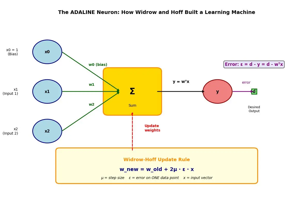
The diagram above shows the ADALINE (Adaptive Linear Neuron) architecture. Inputs x0, x1, x2 come in. Each is multiplied by a weight (w0, w1, w2). The neuron sums them up to produce output y. The error is calculated as ε = d − y (desired minus actual). This error is fed back to update the weights. This loop repeats until the error is minimized.
Here is how ADALINE works:
- Inputs arrive: x0 (always 1, for the bias), x1, x2, etc.
- Weighted sum: y = w0·x0 + w1·x1 + w2·x2 = wᵀx
- Compare with desired output d: error ε = d − y
- Update weights: w_new = w_old + 2μ · ε · x
The weight update rule is beautifully simple. It says: "Adjust each weight by a small amount proportional to the error and the input." If the error is large, adjust more. If the input was zero, that weight does not need to change (because it did not contribute to the error).
The Letter Recognition Problem
Widrow and Hoff tested their algorithm on a fun problem: teaching a machine to recognize letters. They used a 4×4 grid of pixels — 16 pixels total, each either black (1) or white (0). They wanted the machine to distinguish between the letter "T" and the letter "J".
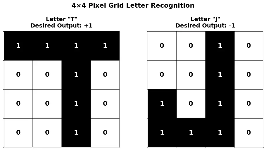
The 4×4 pixel grids for "T" and "J". Each letter is a 16-dimensional vector of 0s and 1s. The machine must learn weights that produce +1 for "T" and −1 for "J".
When "T" is shown, the desired output is +1. When "J" is shown, the desired output is −1. The machine starts with random weights. It sees "T," calculates its output, finds the error, and adjusts. Then it sees "J," calculates, finds error, adjusts again. Back and forth, back and forth — just like the Perceptron, but using the error magnitude to guide the step size.
Widrow and Hoff built a physical ADALINE machine using electronic parts they bought from a local electronics store in Palo Alto. They spent the whole weekend soldering and testing. By Sunday afternoon, it worked! They called it ADALINE — ADAptive LInear NEuron.
Later, Widrow built MADALINE — Many ADALINEs — a network with three layers: input, hidden, and output. This was one of the first multi-layer neural networks. But training it was hard, and the field of neural networks would soon enter a long winter.
6. The LMS Algorithm: The Math Made Simple
Let us look at the LMS update rule more carefully. The book gives us:
w_new = w_old + 2μ · ε · x
Where:
- μ (mu) = step size (learning rate)
- ε (epsilon) = error = d − wᵀx (desired output minus actual output)
- x = input vector
Why Does This Work?
Think of the error ε as a measure of how unhappy we are. If ε is positive, the actual output is too small — we need to increase the weights. If ε is negative, the actual output is too big — we need to decrease the weights.
The term ε · x tells us exactly how to adjust each weight. If input x_i was large and the error was large, weight w_i gets a big adjustment. If x_i was zero, that weight does not change — it was not responsible for the error.
The factor 2μ controls how aggressively we adjust. Small μ = cautious learning. Large μ = bold learning (but risk of overshooting).
The "Noisy" Gradient
Here is the most brilliant insight from Widrow and Hoff. Normally, to do gradient descent properly, you need to calculate the average error over ALL data points. This is expensive and requires calculus.
Widrow and Hoff said: "Forget the average. Just use ONE data point. Calculate the error for that single point. Update the weights. Move to the next point."
This gives a very noisy, approximate gradient. As Widrow later joked: "You take the single value of the error, square it, swallow hard, because you are going to tell a lie, and you say that's the mean squared error. It's a pretty noisy version of the average."
But here is the miracle: it works anyway. If you take enough small steps, the noise averages out. The steps wander around like a drunk person, but they drift steadily toward the bottom of the bowl.
This is now called Stochastic Gradient Descent (SGD), and it is the algorithm used to train virtually every deep neural network in the world.
7. The History: From Blackboards to Billions
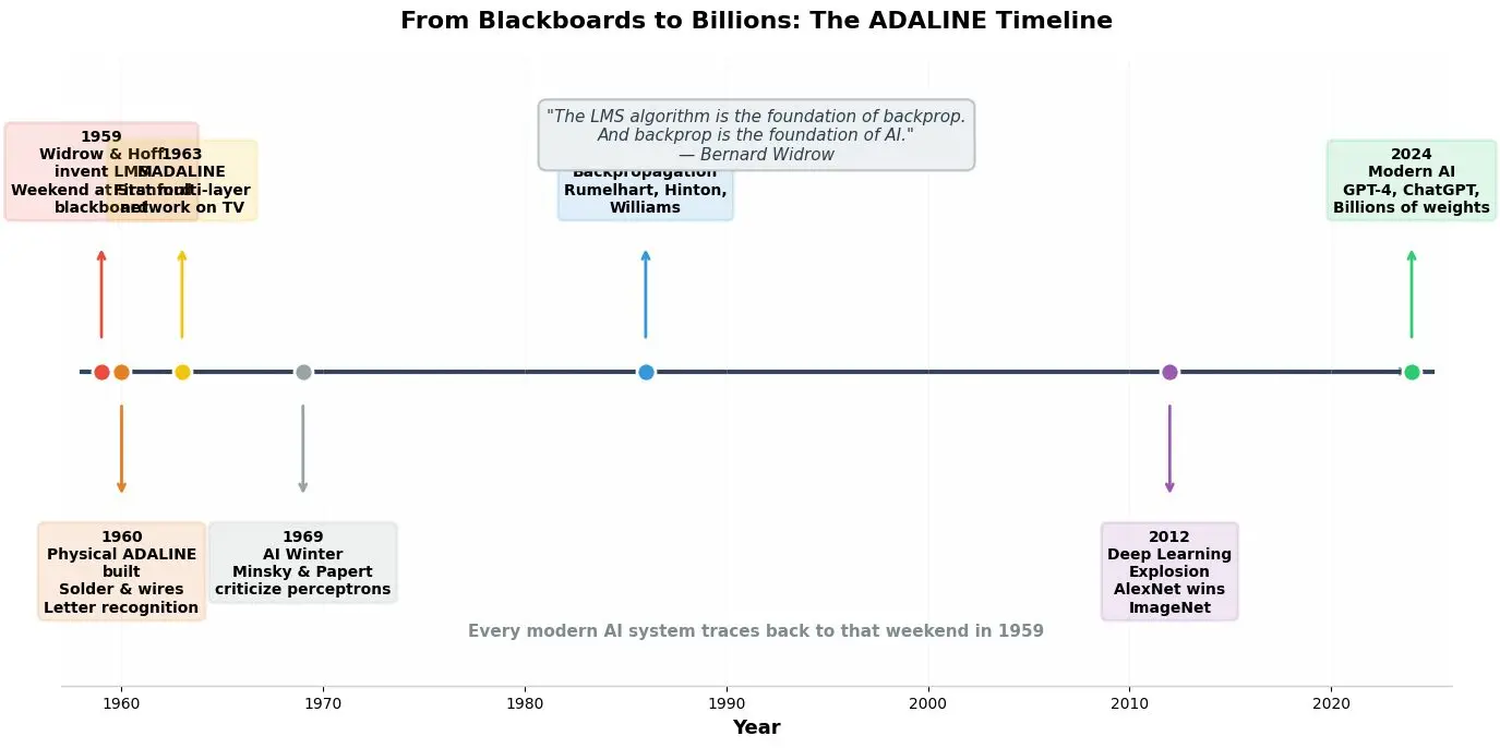
The timeline shows the incredible journey from 1959 to today. Widrow and Hoff invented LMS in 1959. They built ADALINE in 1960. MADALINE followed in 1963. Then came the AI winter, followed by the backpropagation revolution in 1986, and finally the deep learning explosion with AlexNet in 2012. Every modern AI system traces back to that weekend in 1959.
The Key Events
- 1959: Widrow and Hoff invent LMS over a weekend at Stanford. Hoff later admits: "Foolishly I was thinking: 'We've discovered the secret of life.'"
- 1960: They build the physical ADALINE machine. It learns to recognize letters using knobs and wires.
- 1963: MADALINE — a three-layer network — is demonstrated on TV. The host asks Widrow why it is called "ADALINE" and not a masculine name. Widrow replies: "Well, this happens to spell 'Adaptive Linear Neuron.' And that's it."
- 1969: Minsky and Papert publish Perceptrons, criticizing the limitations of single-layer networks. Neural network research enters a long winter.
- 1986: Backpropagation is popularized by Rumelhart, Hinton, and Williams. The LMS idea is extended to multiple layers.
- 2012: AlexNet wins the ImageNet competition, sparking the deep learning revolution. Modern networks have millions or billions of weights.
- Today: Every deep neural network — ChatGPT, image generators, self-driving cars — uses some form of gradient descent. The foundation was laid by two men on a blackboard in 1959.
Widrow's Prophetic Words
In the book, Widrow says something extraordinary:
"The LMS algorithm is the foundation of backprop. And backprop is the foundation of AI. In other words, if you trace it back, this whole field of AI right now, [it] all starts with ADALINE."
This is not an exaggeration. When you train a modern neural network with billions of weights, the core idea is still: calculate the error, find the gradient, take a small step in the direction that reduces the error. That is LMS. That is gradient descent. That is the bottom of the bowl.
8. Try It Yourself: ADALINE in Pure Python
Below is a complete implementation of the LMS/ADALINE algorithm in pure Python — no NumPy, no sklearn. It includes two examples: learning a straight line, and recognizing letters.
```
python
# ============================================
# ADALINE / LMS ALGORITHM - Pure Python
# No numpy, no sklearn!
# Based on Widrow & Hoff's 1959 invention
# ============================================
def dot_product(a, b):
return sum(x * y for x, y in zip(a, b))
def vector_add(a, b):
return [x + y for x, y in zip(a, b)]
def scalar_multiply(s, v):
return [s * x for x in v]
def lms_train(data, desired_outputs, step_size=0.1, max_iterations=1000):
"""
LMS (Least Mean Squares) Algorithm - Widrow & Hoff
data: list of input vectors
desired_outputs: list of desired values (d)
step_size: learning rate (mu)
max_iterations: safety limit
Returns: learned weights
"""
num_features = len(data[0])
w = [0.0] * num_features # Start with zero weights
print("=" * 60)
print("ADALINE / LMS ALGORITHM - Widrow & Hoff (1959)")
print("=" * 60)
print(f"Step size (μ): {step_size}")
print(f"Number of features: {num_features}")
print("Step 1: Starting with all weights = 0")
print("-" * 60)
for iteration in range(max_iterations):
total_error = 0
for i, (x, d) in enumerate(zip(data, desired_outputs)):
# Calculate output
y = dot_product(w, x)
# Calculate error
error = d - y
total_error += error ** 2
# Update weights: w_new = w_old + 2*mu*error*x
update = scalar_multiply(2 * step_size * error, x)
w = vector_add(w, update)
# Print progress every 100 iterations
if iteration % 100 == 0:
print(f"Iteration {iteration}: Total Squared Error = {total_error:.6f}")
print(f" Weights: {[round(v, 4) for v in w]}")
# Check convergence
if total_error < 0.001:
print(f"\nCONVERGED at iteration {iteration}!")
print(f"Final weights: {[round(v, 4) for v in w]}")
return w
print(f"\nReached max iterations. Final error: {total_error:.6f}")
return w
def predict(w, x):
"""Make prediction with trained ADALINE."""
return dot_product(w, x)
# ============================================
# EXAMPLE 1: Simple Linear Regression
# Predicting a line: y = 2x + 1
# ============================================
print("\n" + "=" * 60)
print("EXAMPLE 1: Learning a Straight Line")
print("=" * 60)
print("We want the machine to learn: y = 2x + 1")
print()
# Training data: [bias=1, x], desired_output = 2x + 1
training_data = [
[1.0, 0.0], # y = 1
[1.0, 1.0], # y = 3
[1.0, 2.0], # y = 5
[1.0, 3.0], # y = 7
[1.0, 4.0], # y = 9
]
desired = [1.0, 3.0, 5.0, 7.0, 9.0]
weights = lms_train(training_data, desired, step_size=0.05, max_iterations=500)
print("\n--- Testing the learned line ---")
test_points = [
[1.0, 5.0], # Should predict 11
[1.0, -1.0], # Should predict -1
]
for x in test_points:
pred = predict(weights, x)
print(f"Input x={x[1]}: Predicted y = {pred:.2f} (Expected: {2*x[1]+1})")
# ============================================
# EXAMPLE 2: Letter Recognition (T vs J)
# 4x4 pixel grid = 16 features + 1 bias = 17 weights
# ============================================
print("\n" + "=" * 60)
print("EXAMPLE 2: Recognizing Letters T and J")
print("=" * 60)
# Letter T: 4x4 grid flattened (row by row)
letter_T = [1.0] + [1,1,1,1, 0,0,1,0, 0,0,1,0, 0,0,1,0]
# Letter J: 4x4 grid flattened
letter_J = [1.0] + [0,0,1,0, 0,0,1,0, 1,0,1,0, 1,1,1,0]
letter_data = [letter_T, letter_J]
letter_desired = [1.0, -1.0] # T = +1, J = -1
letter_weights = lms_train(letter_data, letter_desired, step_size=0.01, max_iterations=1000)
print("\n--- Testing letter recognition ---")
for name, letter, expected in [("T", letter_T, 1.0), ("J", letter_J, -1.0)]:
pred = predict(letter_weights, letter)
classification = "T" if pred > 0 else "J"
print(f"Letter {name}: Output = {pred:.4f} → Classified as {classification}")
# Test with a slightly noisy T
noisy_T = [1.0] + [1,1,1,1, 0,0,1,0, 0,0,1,0, 0,0,0,0] # Last pixel changed
pred_noisy = predict(letter_weights, noisy_T)
print(f"\nNoisy T (one pixel wrong): Output = {pred_noisy:.4f} → Classified as {'T' if pred_noisy > 0 else 'J'}")
```
When you run this code, you will see the machine start with zero weights and gradually learn. In Example 1, it discovers the line y = 2x + 1 by minimizing the squared error. In Example 2, it learns to distinguish "T" from "J" using 17 weights. Even if you give it a slightly damaged "T," it still classifies it correctly — because it has learned the pattern, not just memorized the pixels.
9. Summary: The Big Picture
Let us step back and see what we have learned in this blog.
The Core Idea: Learning as Descent
Machine learning is not magic. It is optimization. We define an "error bowl" — a function that measures how wrong our machine is. The bottom of the bowl is the place where the error is smallest — the best possible answer. We start somewhere on the side of the bowl. We calculate the slope (gradient) at our current position. We take a small step in the direction that reduces the error. We repeat until we reach the bottom.
The Rice Terrace → The Math → The Machine
The book beautifully connects these three levels:
- Intuition: Walking down rice terraces in Vietnam — feeling the slope, taking small steps.
- Mathematics: The bowl y = x², derivatives, partial derivatives, gradient vectors.
- Engineering: ADALINE, the LMS algorithm, physical neurons built with solder and wires.
From 3 Weights to Billions
Widrow and Hoff started with 3 weights. Today, GPT-4 has an estimated 1.8 trillion weights. But the algorithm is the same: calculate error, find gradient, take a small step. The scale has changed by a factor of a billion, but the mathematics has not changed at all.
Why This Matters for Beginners
If you are new to machine learning, you might feel overwhelmed by the complexity of modern AI. But remember: at its heart, every learning machine is just a person walking down a hillside in the dark. You cannot see the destination. But you can feel which way is down. And if you keep walking, you will get there.
10. Reference
Anil Ananthaswamy, Why Machines Learn: The Elegant Math Behind Modern AI (2024)
More Machine-Learning tutorials
- Introduction to Machine Learning
- Introduction to Deep Learning
- A Beginner's Guide to Machine Learning
- The First Artificial Neuron and Learning from Mistakes
- Patterns
- Understanding Vectors, the Building Blocks of AI
All tutorials · Try the free PySpark compiler · Practice challenges