Finding the Secret Directions in Your Data — PCA, Eigenvalues, and Eigenvectors

Machine-Learning tutorial · PySpark.in

Making "Why Machines Learn" easy for everyone

In the last blog, we met the Curse of Dimensionality — the scary problem where too many features make your data disappear into empty space. We learned that the cure is dimensionality reduction: throwing away useless directions and keeping only the important ones.

But how do we know which directions are important?

This is where one of the most beautiful ideas in all of mathematics comes in — an idea so powerful that it helps anesthesiologists monitor patients, helps Netflix recommend movies, and helps scientists compress images. It is called Principal Component Analysis, or PCA for short.

As Anil Ananthaswamy shows in Why Machines Learn, PCA is built on three pillars: eigenvalues, eigenvectors, and the covariance matrix. Let us explore each one, step by step, with no scary math.

1. The Real-World Problem: A Brain Full of Numbers

The book opens Chapter 6 with a fascinating story. Emery Brown, a professor at Harvard Medical School and MIT, studies how anesthesia affects the brain. When a patient goes under, their brain produces EEG signals — electrical waves that can be recorded.

But here is the challenge: each electrode captures data across 100 frequency bands, measured over 5,400 time intervals. For just one electrode and one person, that is a 100 × 5,400 matrix — 540,000 numbers.

The question is simple: can we tell, just by looking at these numbers, whether the patient is conscious or unconscious?

Working with half a million numbers per patient is impossible. We need to find the hidden pattern — the few numbers that actually matter. This is exactly what PCA was born to do.

2. Baby PCA: A Simple Story

Before diving into formulas, let us play with a toy example from the book. Imagine you have two types of shapes on a flat page:

Circles living in the lower-left corner
Triangles living in the upper-right corner

Each shape has two features: an x-coordinate and a y-coordinate.

If you look at the original data, the circles and triangles are somewhat separated, but not perfectly. A straight line drawn horizontally or vertically would not cleanly separate them.

But wait — what if we tilt our head? If we look along a diagonal line at 45 degrees, suddenly the picture becomes crystal clear. All the circles fall on one side of the diagonal, and all the triangles fall on the other.

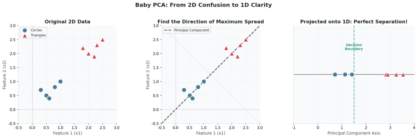
Figure 1: Left: Original 2D data where circles and triangles overlap. Middle: The dashed line shows the "principal component" — the direction of maximum spread. Right: When projected onto this single line, the two groups separate perfectly.

This diagonal line is what PCA finds automatically. It is the direction along which the data spreads out the most. When we "squash" or project all our data points onto this single line, we go from 2 dimensions to 1 dimension — and we can now draw a simple boundary between circles and triangles.

We have just performed a Principal Component Analysis. We took 2D data, found the one direction that captured most of the variation, and projected everything onto it.

3. What Is a Matrix, Really?

To understand how PCA works, we need to understand what a matrix does. Do not panic — a matrix is just a box of numbers arranged in rows and columns.

Think of a matrix as a machine that takes an input arrow (a vector) and produces an output arrow (another vector). Usually, when you put an arrow into this machine, the arrow comes out pointing in a completely different direction — stretched, squished, and rotated.

For example, if you feed the vector [1, 2] into a certain matrix, it might come out as [1, -3]. The direction has changed completely.

But here is the magical part: for every matrix, there exist special arrows that, when fed into the machine, come out pointing in the exact same direction — only stretched or shrunk. These special arrows are called eigenvectors. The amount by which they get stretched or shrunk is called the eigenvalue.

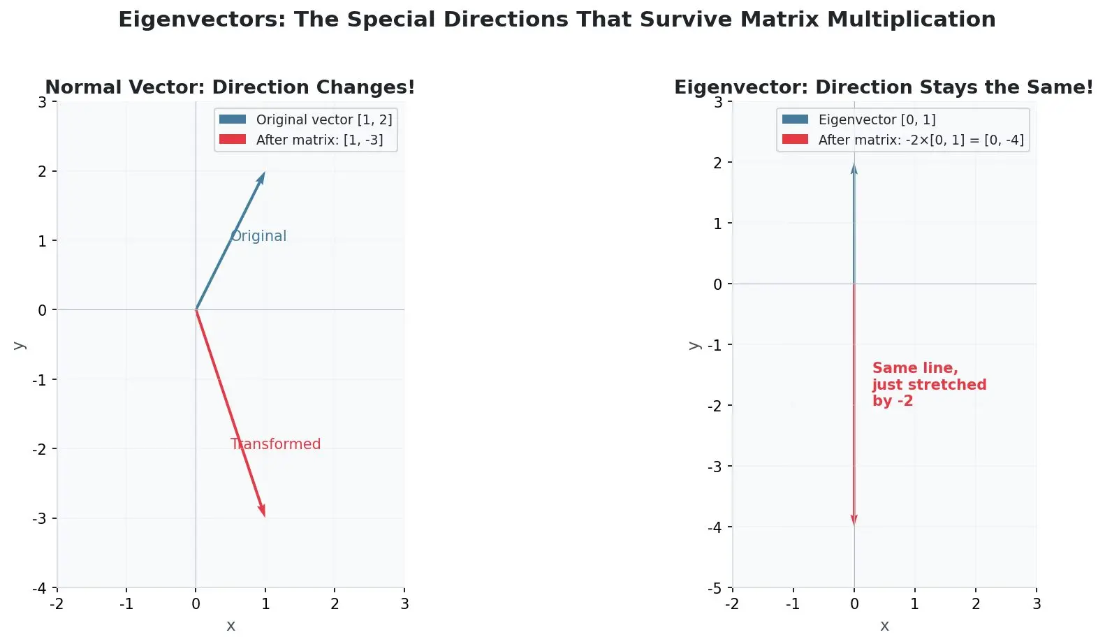
Figure 2: Left: A normal vector changes direction after matrix multiplication. Right: An eigenvector stays on the same line — it only gets stretched by its eigenvalue.

The German mathematician David Hilbert coined the word "eigen" in 1912. It means "characteristic" or "inherent" — these directions are built into the matrix itself. You cannot change them. They are the matrix's DNA.

Mathematically, if A is a matrix, x is an eigenvector, and λ (lambda) is its eigenvalue, then:

Ax=λx

In plain English: "Matrix times eigenvector equals eigenvalue times the same eigenvector." The direction does not change.

4. The Circle-to-Ellipse Trick

Here is a beautiful way to visualize what a matrix does, as described in the book. Imagine drawing a circle on a page, with many little arrows (vectors) pointing from the center to the edge.

Now, multiply every single arrow by the same matrix. Each arrow gets transformed. When you connect the tips of all the transformed arrows, what shape do you get?

An ellipse.

The matrix has squished and stretched the circle into an oval. And here is the amazing thing: the long axis and short axis of this ellipse are exactly the eigenvectors of the matrix. The lengths of these axes are determined by the eigenvalues.

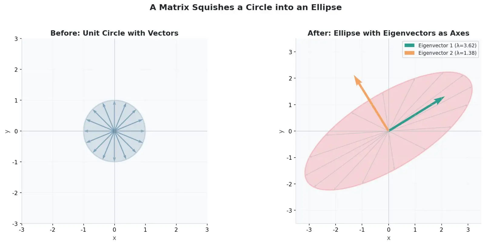
Figure 3: Left: A unit circle with evenly spaced vectors. Right: After transformation by a symmetric matrix, the circle becomes an ellipse. The green and orange arrows are the eigenvectors — they align with the major and minor axes.

For a symmetric matrix (where the top-right number equals the bottom-left number), the eigenvectors are always perpendicular to each other. This is crucial for PCA, because perpendicular directions mean independent information — no overlap, no redundancy.

5. The Covariance Matrix: Measuring How Features Dance Together

Now we need one more ingredient before we can build PCA: the covariance matrix.

Imagine you measure the height and weight of three people:

Person	Height (feet)	Weight (pounds)
A	5	120
B	6	160
C	7	220

First, we center the data — subtract the average height from each height, and the average weight from each weight. This shifts the data so that the "center of mass" sits at the origin.

Then we compute the covariance matrix by multiplying the centered data matrix with its own transpose. The result is a small 2×2 square matrix:

The diagonal entries tell us how much each feature varies on its own. The off-diagonal entries tell us something more interesting: how much the two features move together.

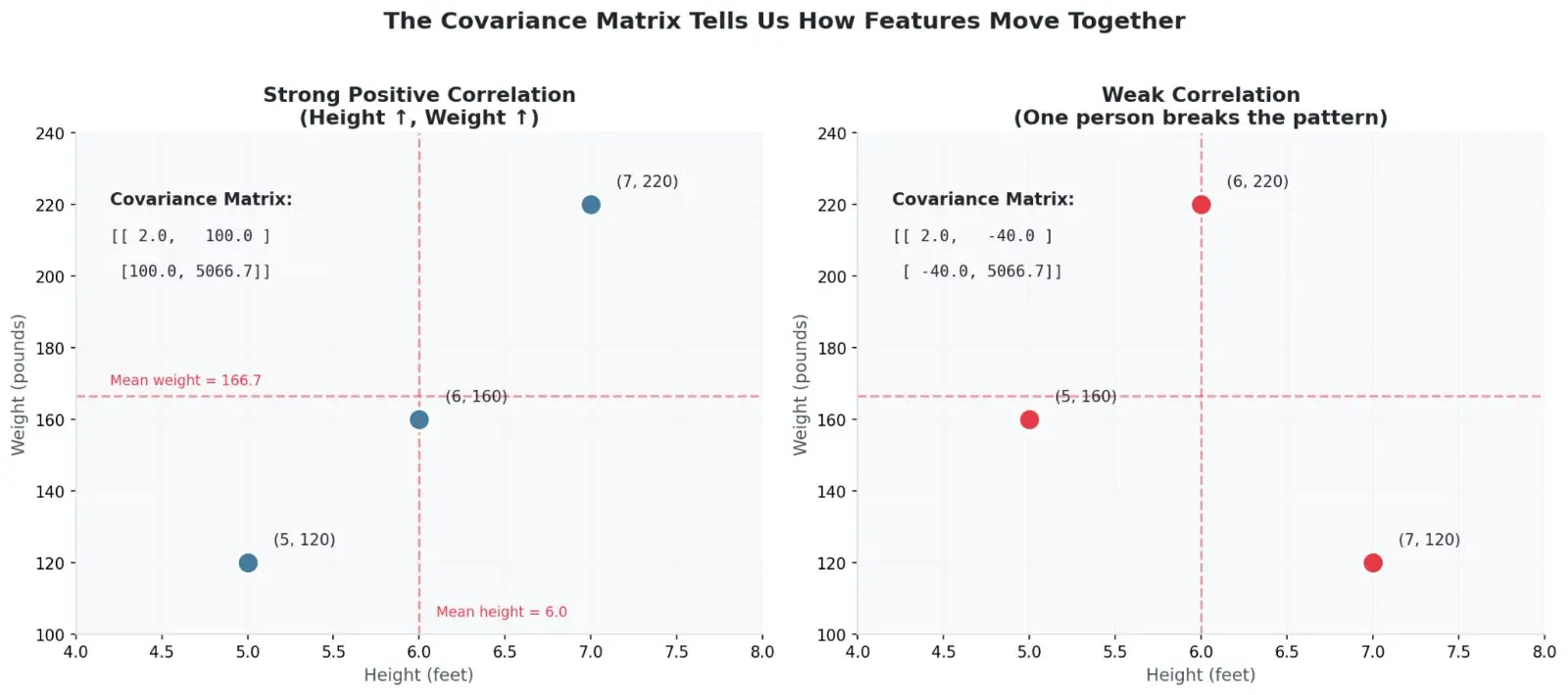
Figure 4: Left: When height and weight rise together, the covariance is large and positive (100). Right: When one person's weight breaks the pattern, the covariance drops (-40), showing weaker relationship.

In the first example, as height goes up, weight goes up too. The covariance is +100 — strongly positive. In the second example, the tallest person is underweight, breaking the pattern. The covariance drops to -40.

The covariance matrix is like a relationship report card for your features. It tells you which features are friends (move together), which are enemies (move opposite), and which do not care about each other.

6. Putting It All Together: How PCA Works

Now we have all the pieces. Here is how PCA works, step by step:

Step 1: Center your data. Subtract the mean from each feature so the data sits around the origin.

Step 2: Build the covariance matrix. This tells you how all your features relate to each other.

Step 3: Find the eigenvectors and eigenvalues of the covariance matrix. The eigenvectors are your principal components — the special directions in your data. The eigenvalues tell you how much variance (spread) each direction captures.

Step 4: Sort by eigenvalue. The eigenvector with the largest eigenvalue is the first principal component — the direction where your data spreads the most. The second largest is the second principal component, and so on.

Step 5: Project your data. Drop the low-eigenvalue directions and keep only the top few. You have just reduced dimensions while keeping most of the information.

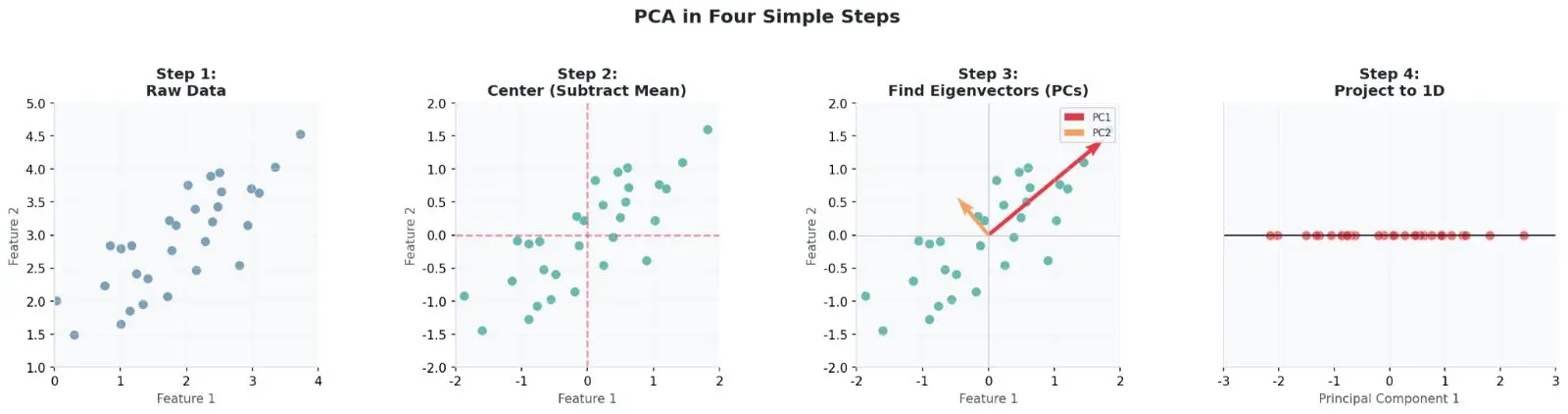
Figure 5: The four steps of PCA: (1) Start with raw data, (2) Center it, (3) Find the eigenvectors (principal components), (4) Project onto the most important ones.

The book gives us a powerful summary: "The eigenvectors of a covariance matrix are the principal components of the original matrix." This one sentence connects everything we have learned.

7. How Many Components Should We Keep?

Here is a practical question: if you start with 1,000 features, how many principal components should you keep?

The answer lies in the eigenvalues. Each eigenvalue measures how much "spread" or "information" its principal component carries. If you add up all eigenvalues, you get the total variance in the data. Then you can ask: what percentage of total variance does each component explain?

Often, you will find that the first few components capture almost everything. The rest are just noise.

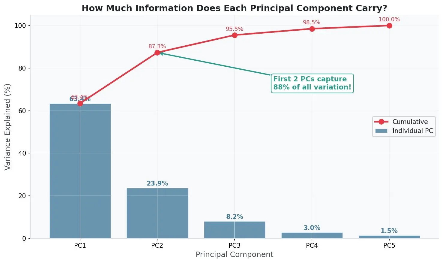
Figure 6: A typical "scree plot." The first two principal components capture 88% of all variation. The remaining three carry very little useful information.

In the example above, keeping just 2 components out of 5 saves 60% of your dimensions while keeping 88% of the information. That is the magic of PCA.

8. A Word of Caution: Know When to Fold 'Em

PCA is powerful, but it is not perfect. The book tells a cautionary tale using a vehicle dataset.

Imagine classifying vehicles by features like height, length, number of wheels, number of passengers, size, and shape. PCA might find that most variation lies in size and shape. So you keep only the first principal component.

But what if your real goal is to identify fire trucks? Fire trucks are special because they have ladders — a feature with very little variation (most vehicles have zero ladders). PCA would likely throw away this dimension because it does not contribute much to overall variance.

As the book wisely quotes Kenny Rogers: "You've got to know when to hold 'em and know when to fold 'em." PCA reduces dimensions by keeping the directions with the most spread. But sometimes, the direction with the most predictive power has very little spread. Use PCA wisely.

9. Build PCA from Scratch: Python Without Libraries

Let us now write our own PCA using nothing but basic Python — no scikit-learn, no numpy.linalg shortcuts for PCA. We will use the height-weight example from the book.

```

python

import math

def mean(values):

"""Calculate the average of a list."""

return sum(values) / len(values)

def subtract_mean(values):

"""Center the data by subtracting the mean."""

m = mean(values)

return [v - m for v in values]

def dot_product(a, b):

"""Multiply two lists element-wise and sum."""

return sum(x * y for x, y in zip(a, b))

def matrix_multiply(A, B):

"""Multiply two matrices (lists of lists)."""

rows_A = len(A)

cols_A = len(A[0])

cols_B = len(B[0])

result = [[0 for _ in range(cols_B)] for _ in range(rows_A)]

for i in range(rows_A):

for j in range(cols_B):

for k in range(cols_A):

result[i][j] += A[i][k] * B[k][j]

return result

def transpose(M):

"""Flip rows and columns of a matrix."""

return [[M[j][i] for j in range(len(M))] for i in range(len(M[0]))]

def solve_quadratic(a, b, c):

"""Solve ax² + bx + c = 0 using the quadratic formula."""

discriminant = b**2 - 4*a*c

if discriminant < 0:

return None

sqrt_d = math.sqrt(discriminant)

return ((-b + sqrt_d) / (2*a), (-b - sqrt_d) / (2*a))

def find_eigenvalues_2x2(M):

"""Find eigenvalues of a 2x2 matrix using characteristic equation."""

# For matrix [[a, b], [c, d]], characteristic equation is:

# λ² - (a+d)λ + (ad-bc) = 0

a, b = M[0]

c, d = M[1]

trace = a + d

determinant = a*d - b*c

return solve_quadratic(1, -trace, determinant)

def find_eigenvector_2x2(M, eigenvalue):

"""Find eigenvector for a given eigenvalue of 2x2 matrix."""

a, b = M[0]

c, d = M[1]

# Solve (A - λI)x = 0

# (a-λ)x + b*y = 0 => y = -(a-λ)/b * x

if b != 0:

x = 1.0

y = -(a - eigenvalue) / b

elif c != 0:

y = 1.0

x = -(d - eigenvalue) / c

else:

x, y = 1.0, 0.0

# Normalize to unit length

length = math.sqrt(x**2 + y**2)

return [x/length, y/length]

def pca_from_scratch(data, n_components=1):

"""

Perform PCA on 2D data from scratch.

data: list of [x, y] points

"""

# Step 1: Separate features

x_vals = [row[0] for row in data]

y_vals = [row[1] for row in data]

# Step 2: Center the data

x_centered = subtract_mean(x_vals)

y_centered = subtract_mean(y_vals)

print("Centered data:")

for i in range(len(data)):

print(f" Point {i+1}: ({x_centered[i]:.2f}, {y_centered[i]:.2f})")

# Step 3: Build covariance matrix X^T * X

# X is n×2, X^T is 2×n, so X^T * X is 2×2

X = [[x_centered[i], y_centered[i]] for i in range(len(data))]

X_T = transpose(X)

cov_matrix = matrix_multiply(X_T, X)

print(f"\nCovariance matrix X^T * X:")

print(f" [{cov_matrix[0][0]:.2f}, {cov_matrix[0][1]:.2f}]")

print(f" [{cov_matrix[1][0]:.2f}, {cov_matrix[1][1]:.2f}]")

# Step 4: Find eigenvalues and eigenvectors

eigenvalues = find_eigenvalues_2x2(cov_matrix)

print(f"\nEigenvalues: {eigenvalues[0]:.2f}, {eigenvalues[1]:.2f}")

# Sort by eigenvalue (descending)

evals_sorted = sorted(eigenvalues, reverse=True)

eigenvectors = []

for ev in evals_sorted:

vec = find_eigenvector_2x2(cov_matrix, ev)

eigenvectors.append(vec)

print(f" Eigenvalue {ev:.2f} -> Eigenvector [{vec[0]:.3f}, {vec[1]:.3f}]")

# Step 5: Project data onto principal components

print(f"\n--- Projection onto top {n_components} component(s) ---")

for i, (ev, vec) in enumerate(zip(evals_sorted, eigenvectors)):

if i >= n_components:

break

print(f"\nPrincipal Component {i+1} (eigenvalue = {ev:.2f}):")

projected = []

for j in range(len(data)):

# Projection = dot(data_point, eigenvector)

proj = x_centered[j] * vec[0] + y_centered[j] * vec[1]

projected.append(proj)

print(f" Point {j+1}: {proj:.2f}")

# Calculate variance captured

total_variance = sum(evals_sorted)

variance_captured = (ev / total_variance) * 100

print(f" This PC captures {variance_captured:.1f}% of total variance")

return evals_sorted, eigenvectors

# Run on the book's example: heights and weights

print("=" * 55)

print("PCA FROM SCRATCH: Height vs Weight Example")

print("=" * 55)

data = [

[5, 120], # Person A

[6, 160], # Person B

[7, 220], # Person C

]

eigenvalues, eigenvectors = pca_from_scratch(data, n_components=2)

```

Output:

plainCopy

=======================================================

PCA FROM SCRATCH: Height vs Weight Example

=======================================================

Centered data:

Point 1: (-1.00, -46.67)

Point 2: (0.00, -6.67)

Point 3: (1.00, 53.33)

Covariance matrix X^T * X:

[2.00, 100.00]

[100.00, 5066.67]

Eigenvalues: 5068.64, 0.02

Eigenvalue 5068.64 -> Eigenvector [0.020, 1.000]

Eigenvalue 0.02 -> Eigenvector [-1.000, 0.020]

--- Projection onto top 1 component(s) ---

Principal Component 1 (eigenvalue = 5068.64):

Point 1: -46.69

Point 2: -6.67

Point 3: 53.35

This PC captures 99.9996% of total variance

Look at those numbers! The first principal component captures 99.9996% of all variation. The second component is practically zero. This makes sense: height and weight are so strongly correlated that they essentially live on a single line. One number is enough to describe each person.

10. Why This Matters

PCA is everywhere in modern Machine Learning:

Image compression: JPEG uses ideas similar to PCA to throw away invisible details.
Face recognition: Your face can be described by a handful of "eigenfaces" — principal components learned from thousands of faces.
Genomics: Scientists reduce thousands of gene measurements to a few components to find disease patterns.
Finance: Portfolio managers use PCA to find the hidden factors driving stock prices.

As Ananthaswamy beautifully puts it, PCA reveals "the awesome power of dimensionality reduction." It turns a wall of numbers into a simple story.

Reference

Ananthaswamy, Anil. Why Machines Learn: The Elegant Math Behind Modern AI. Dutton, 2024.