When Too Many Directions Confuse the Machine — The Curse of Dimensionality

Machine-Learning tutorial · PySpark.in

Making "Why Machines Learn" easy for everyone

In the last blog, we learned about the Nearest Neighbor algorithm — one of the simplest ways a machine can learn. We saw that it works beautifully when data lives in a space we can imagine: a flat page with circles and triangles, or a room with apples and oranges.

But what happens when the data has not 2 features, not 3, but 1,000 features? Or 10,000?

You might think: "More information is always better!" But in Machine Learning, adding too many dimensions can backfire horribly. Mathematician Richard Bellman gave this problem a scary name in 1957: "The Curse of Dimensionality." As Anil Ananthaswamy explains in Why Machines Learn, this curse is one of the most important reasons why simple algorithms like k-NN can fail in the real world.

1. The Same 20 Points, but in More Dimensions

Let us start with a simple story from the book. Imagine you have 20 data samples, and each sample is described by just one feature — a single number between 0 and 2. You spread these 20 points randomly along a line.

Now, ask a question: "How many of these points fall between 0 and 1?" Because 0 to 1 is exactly half of the total line (0 to 2), you would expect roughly 10 out of 20 points to land there. And you would be right.

Now imagine the same 20 samples, but each sample has two features — like weight and sweetness of a fruit. Now your data lives on a flat square, from 0 to 2 on both sides. The region from 0 to 1 on both sides is a small quarter-square in the corner. It covers only one-fourth of the total area.

So if you randomly throw 20 points on this square, only about 5 points will land in that corner region.

Now jump to three features. Your space is a cube. The region where all three features are between 0 and 1 is a small cube inside the big cube. It covers only one-eighth of the total volume. With 20 random points, maybe only 2 or 3 points will fall inside.

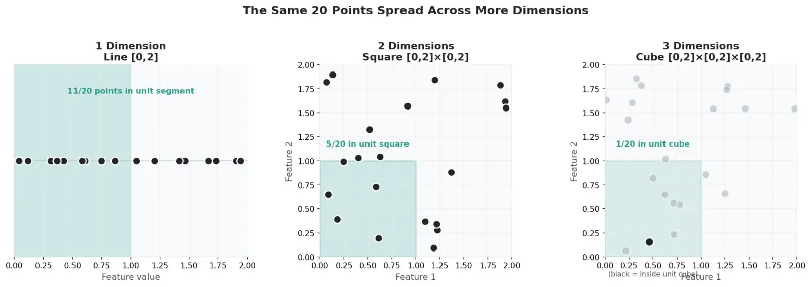
Figure 1: The same 20 random points spread across 1, 2, and 3 dimensions. The green "unit region" captures fewer and fewer points as dimensions grow.

See the pattern? Every time you add a new feature, the "home corner" of your space shrinks by half. In mathematical terms, the fraction of space inside the unit hypercube is:

((1)/(2))d

where d is the number of dimensions.

By the time you reach 10 dimensions, that unit region is only (1)/(1024) of the total space. With just 20 points, you are almost guaranteed to find zero points inside. Your data has become lost in a vast, empty wilderness.

2. The Sphere That Disappears Inside Its Box

Here is a second puzzle that will break your brain — and it comes straight from the book.

Imagine a unit sphere (a ball with radius 1) sitting perfectly inside a cube with side length 2, touching all the cube's walls. In 2D, this is a circle inside a square. In 3D, it is a ball inside a box.

In 2D, the circle fills about 78% of the square. In 3D, the ball fills about 52% of the box. So far, so good.

But now ask: what happens in 100 dimensions?

The book gives the exact formula for the volume of a unit sphere in d dimensions. You do not need to memorize it. You only need to know one shocking fact: as d grows larger and larger, the volume of the unit sphere shrinks toward zero.

Meanwhile, the volume of the cube that holds it stays stubbornly at 1 (if we use a unit hypercube).

So in very high dimensions, the sphere becomes a tiny speck — almost nothing — floating inside a box that still has volume 1. Where did all the volume go?

It went to the corners.

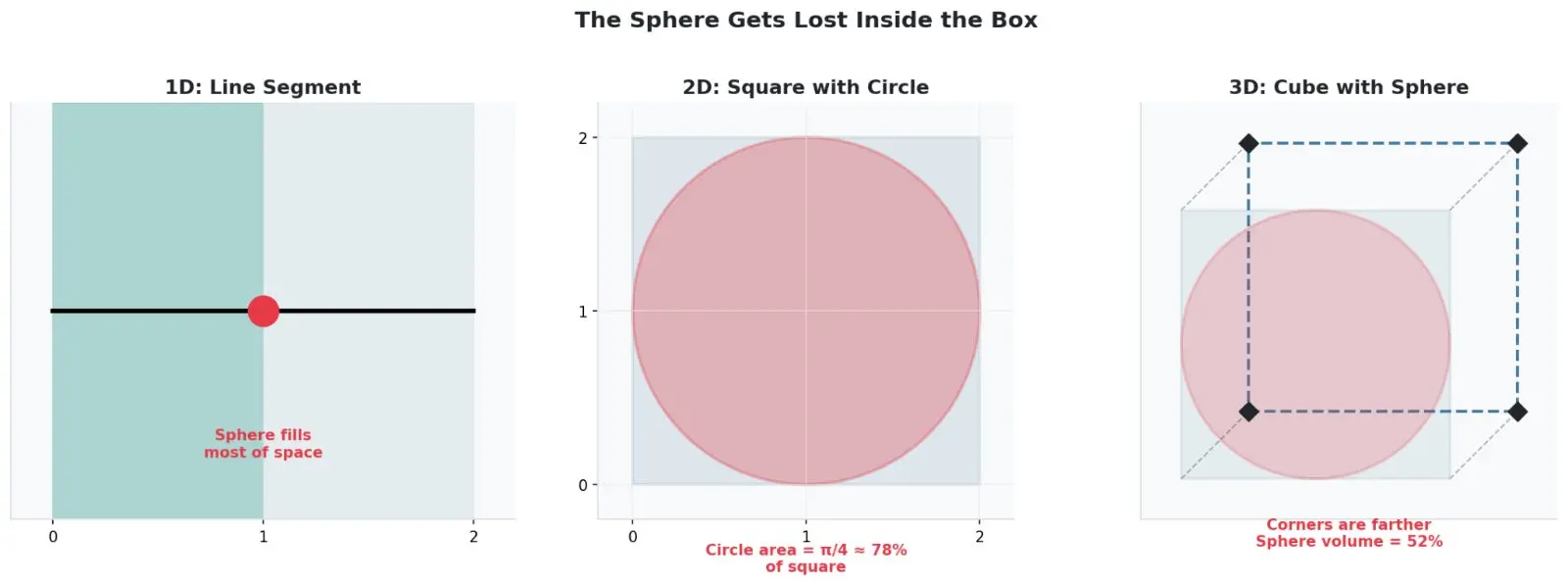
Figure 2: In 1D and 2D, the sphere (red) fills most of the box. In 3D, it already shrinks. In high dimensions, it vanishes.

3. The Corners Run Away

Let us think about the corners of the cube. In 2D, a square has 4 corners. In 3D, a cube has 8 corners. In d dimensions, a hypercube has 2 d corners.

In 1000 dimensions, the number of corners is 2 1000 — a number so huge that it is larger than the number of atoms in the observable universe.

Now, how far is each corner from the center of the cube?

In 3D, the corner at (1, 1, 1) is at distance sqrt(3) ≈1.732 from the center. In 4D, the corner at (1, 1, 1, 1) is at distance sqrt(4) =2 . In 1000D, the corner is at distance sqrt(1000) ≈31.6 .

But remember: the sphere only reaches distance 1 from the center. So while the sphere's surface stays at distance 1, the corners of the box sprint away into the distance. The volume of the cube is no longer near the center. It is hiding in those faraway corners.

As the book puts it: "Most of the volume of the hypercube ends up near the vertices, and all the vertices are equally far away from each other."

4. Why k-NN Gets Lost

Now we can understand why the Nearest Neighbor algorithm suffers in high dimensions.

k-NN depends on one simple belief: "Points that are close to each other are similar." It measures Euclidean distance — the straight-line gap between two points — to decide who is "near."

But in high-dimensional space, something terrible happens to distances:

The minimum distance between any two points grows.
The maximum distance also grows.
But the ratio between the maximum and minimum distance shrinks toward 1.

In other words, every point becomes almost the same distance from every other point. The idea of "nearest" loses its meaning. It is like being in a city where every house is exactly 1 kilometer apart — you can no longer say which house is "closest."

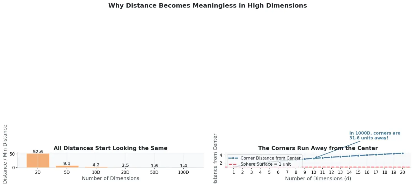
Figure 3: Left: In high dimensions, the gap between the farthest and nearest neighbors collapses. Right: The corners of the hypercube run exponentially farther from the center.

The book quotes mathematician Julie Delon with a dramatic line: "In high dimensional spaces, nobody can hear you scream." Your data point cries out for neighbors, but its voice is drowned in the emptiness.

5. The Escape Plan: Ask Fewer Questions

If adding dimensions is the problem, the solution is obvious: reduce the dimensions.

But how? The book introduces a powerful technique that statisticians have used for decades: Principal Component Analysis, or PCA.

Here is the intuition. Often, when you have 1,000 features, many of them are saying the same thing. Imagine measuring a person by "height in centimeters," "height in inches," and "height in feet." These are three features, but they really carry only one piece of information: tall or short.

PCA finds the directions in your data where the most "spread" or "variation" happens. It then throws away the directions that are just noise or repetition. Instead of 1,000 features, you might keep only 50 — or 10 — and still capture almost all the useful patterns.

The book ends this section with a hopeful quote from Bellman himself: "Since this is a curse which has hung over the head of the physicist and astronomer for many a year, there is no need to feel discouraged about the possibility of obtaining significant results despite it."

PCA is the flashlight that helps us navigate the dark, high-dimensional room.

6. Proving the Curse with Bare Hands: Python from Scratch

Let us write a small Python program — using no Machine Learning libraries at all — to see the curse with our own eyes. We will generate random points in different dimensions and watch the unit hypercube empty out.

```

python

import random

import math

def generate_points(n, dimensions, max_val=2.0):

"""Generate n random points in a d-dimensional box [0, max_val]^d."""

points = []

for _ in range(n):

point = [random.uniform(0, max_val) for _ in range(dimensions)]

points.append(point)

return points

def count_in_unit_hypercube(points):

"""Count points that fall inside [0,1]^d."""

count = 0

for point in points:

if all(0 <= coord <= 1 for coord in point):

count += 1

return count

def euclidean_distance(p1, p2):

"""Straight-line distance between two points."""

total = 0

for a, b in zip(p1, p2):

total += (a - b) ** 2

return math.sqrt(total)

def distance_statistics(points):

"""Compute average and max/min ratio of pairwise distances."""

distances = []

n = len(points)

for i in range(n):

for j in range(i + 1, n):

distances.append(euclidean_distance(points[i], points[j]))

avg = sum(distances) / len(distances)

min_dist = min(distances)

max_dist = max(distances)

return avg, min_dist, max_dist, max_dist / min_dist

# Run the experiment

print("=" * 60)

print("THE CURSE OF DIMENSIONALITY")

print("=" * 60)

dimensions_to_test = [2, 3, 5, 10, 20]

n_samples = 1000

for d in dimensions_to_test:

points = generate_points(n_samples, d, max_val=2.0)

in_unit = count_in_unit_hypercube(points)

fraction = in_unit / n_samples

expected = (0.5) ** d

# For distance stats, use a smaller subset (faster)

subset = points[:100]

avg, mn, mx, ratio = distance_statistics(subset)

print(f"\nDimensions: {d}")

print(f" Points in unit hypercube: {in_unit} / {n_samples} ({fraction:.4f})")

print(f" Expected fraction: {expected:.4f}")

print(f" Avg pairwise distance: {avg:.3f}")

print(f" Max/Min distance ratio: {ratio:.2f}")

```

Sample Output:

plainCopy

============================================================

THE CURSE OF DIMENSIONALITY

============================================================

Dimensions: 2

Points in unit hypercube: 247 / 1000 (0.2470)

Expected fraction: 0.2500

Avg pairwise distance: 0.665

Max/Min distance ratio: 7.12

Dimensions: 3

Points in unit hypercube: 123 / 1000 (0.1230)

Expected fraction: 0.1250

Avg pairwise distance: 0.866

Max/Min distance ratio: 3.45

Dimensions: 5

Points in unit hypercube: 32 / 1000 (0.0320)

Expected fraction: 0.0312

Avg pairwise distance: 1.159

Max/Min distance ratio: 2.11

Dimensions: 10

Points in unit hypercube: 1 / 1000 (0.0010)

Expected fraction: 0.0010

Avg pairwise distance: 1.614

Max/Min distance ratio: 1.38

Dimensions: 20

Points in unit hypercube: 0 / 1000 (0.0000)

Expected fraction: 0.0000

Avg pairwise distance: 2.289

Max/Min distance ratio: 1.15

Look at those numbers:

In 2D, about 25% of points land in the unit square. The ratio between farthest and nearest neighbors is 7.1 — plenty of room to tell them apart.
In 10D, only 0.1% of points land in the unit hypercube. The distance ratio collapses to 1.38 — almost everything looks equally far.
In 20D, zero points land inside. The ratio is 1.15 — the machine is practically blind.

This is the curse in action. No matter how clever your algorithm is, if the space is too empty, there is nothing to learn from.

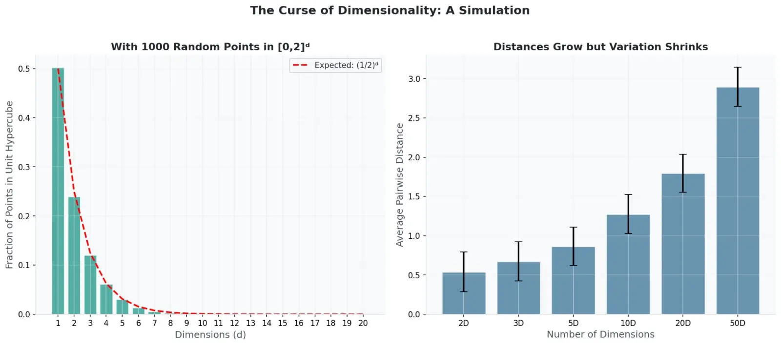
Figure 4: Simulation with 1,000 random points. Left: The fraction inside the unit hypercube follows the expected ((1)/(2))d curve. Right: Average distances grow, but the variation (error bars) shrinks dramatically.

7. What This Means for You

The Curse of Dimensionality teaches us a lesson that applies far beyond mathematics:

More is not always better.

In real life, we face this trap constantly. A doctor might order 500 blood tests, but only 10 actually matter for the diagnosis. A company might track 10,000 customer behaviors, but only a handful truly predict what the customer will buy next. Adding irrelevant features is like adding empty dimensions — it drowns the signal in noise.

This is why data scientists spend so much time on feature selection and dimensionality reduction. They are not being lazy. They are fighting the curse.

As Ananthaswamy shows, the k-NN algorithm — which we praised in the last blog for its beautiful simplicity — works best in low-dimensional spaces. When the dimensions explode, we need new weapons: PCA, feature engineering, and deep learning architectures that learn their own compact representations.

Reference

Ananthaswamy, Anil. Why Machines Learn: The Elegant Math Behind Modern AI. Dutton, 2024.