The Magic Trick That Made Deep Learning Possible: Understanding Backpropagation

Machine-Learning tutorial · PySpark.in

1. The Myth That Held Us Back for 30 Years

For a very long time, scientists believed something that turned out to be completely wrong. They thought that if you built a neural network with more than one layer, it was impossible to train. It was like saying, "You can teach a dog one trick, but you can never teach it a sequence of tricks." This idea was so strong that it became a persistent myth in the world of machine learning.

But in the 1980s, a small group of researchers — Rumelhart, Hinton, and Williams — discovered an algorithm that killed this myth forever. That algorithm is called backpropagation, and it is the reason why your phone can recognize your face, why ChatGPT can write essays, and why doctors can use computers to spot diseases in X-rays.

In this blog, we will learn backpropagation using the simplest possible words. We will not use big libraries. We will build things from scratch. Even if you have never written a line of code in your life, by the end of this blog, you will understand the engine that drives almost all modern artificial intelligence.

2. The Simplest Network: A Baby Brain

To understand backpropagation, we do not need a giant network with millions of neurons. We can understand everything using the smallest possible brain:

One input (let us call it x)
One hidden neuron (the secret worker in the middle)
One output (the final guess, which we call yhat)

Imagine you are trying to predict the price of a house based on its size. You give the network the size (x), the hidden neuron does some math, and the output neuron gives you a predicted price (yhat).

The Forward Pass: Making a Guess

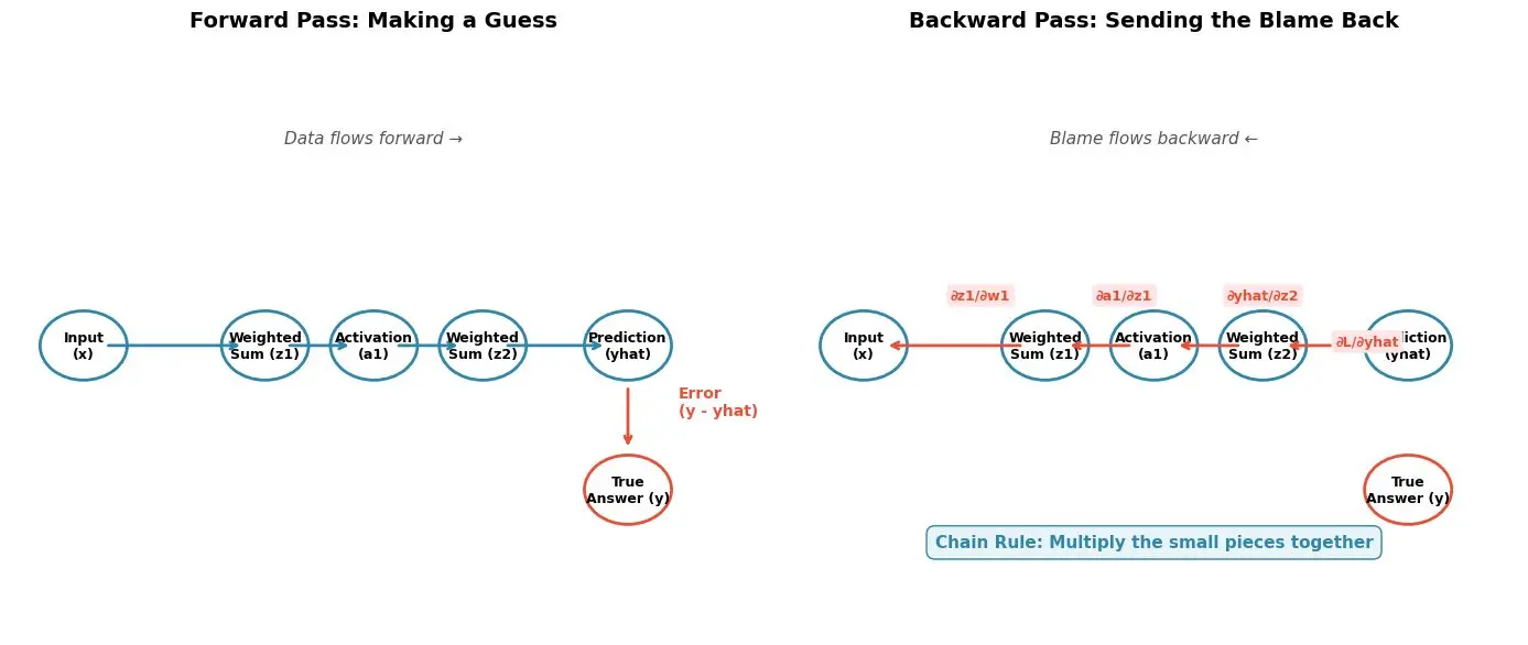
When information moves from left to right, we call it the forward pass. It is like an assembly line in a factory.

Step 1: The hidden neuron takes the input x, multiplies it by a weight (w1), and adds a bias (b1). This gives us a number called z1.

z1 = w1 × x + b1

Think of the weight as "how much I care about the input" and the bias as "my starting opinion before I see anything."

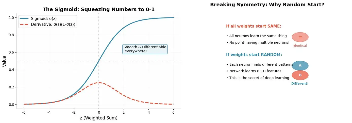
Step 2: We pass z1 through something called an activation function. In our case, we use the sigmoid function, which squishes any number into a value between 0 and 1. We call the result a1.

a1 = sigmoid(z1)

Why do we do this? Because life is not always a straight line. The sigmoid helps the network learn curved, complex patterns instead of just straight-line relationships.

Step 3: The output neuron takes a1, multiplies it by another weight (w2), adds another bias (b2), and gets z2. Then it applies the sigmoid again to get the final prediction.

z2 = w2 × a1 + b2

yhat = sigmoid(z2)

3. The Mistake: How Wrong Was Our Guess?

After the network makes a guess (yhat), we compare it to the true answer (y). The difference is the error:

e = y - yhat

If the true price of the house was $200,000 and we guessed $180,000, our error is $20,000. To make the math cleaner, we define the loss as the square of the error:

Loss = e²

Why square it? Two reasons:

It makes the number positive (so -5 and +5 are equally bad).
It punishes big mistakes much more than small ones.

Our goal is simple: make the Loss as small as possible.

4. The Core Question: Who Is to Blame?

Now we reach the heart of the problem. The network made a mistake. The loss is big. We want to fix it.

But here is the tricky part: Which knob should we turn?

We have four knobs in our tiny network:

w1 (weight in the hidden layer)
b1 (bias in the hidden layer)
w2 (weight in the output layer)
b2 (bias in the output layer)

If we change w2 a little bit, how does the loss change? If we change w1 a little bit, how does the loss change?

We need to know the gradient of the loss with respect to each knob. In simple words: we need to know which direction to turn each knob to make the loss smaller.

5. The Chain Rule: The Whisper Game

To find these gradients, we use something called the chain rule. Do not let the name scare you. It is just a fancy way of saying: if you want to know how a small change at the beginning affects the end, multiply the small effects at each step along the way.

Imagine a line of five people playing a whisper game. You whisper a secret to the first person, they pass it to the second, and so on, until it reaches the last person. If you want to know how much the final message changes when you change your original whisper, you just multiply how much each person changes the message as they pass it along.

Mathematically, if Loss depends on yhat, and yhat depends on z2, and z2 depends on w2, then:

∂Loss / ∂w2 = (∂Loss / ∂e) × (∂e / ∂yhat) × (∂yhat / ∂z2) × (∂z2 / ∂w2)

Let us calculate each small piece:

Loss to Error: Loss = e², so ∂Loss/∂e = 2e
Error to Prediction: e = y - yhat, so ∂e/∂yhat = -1
Prediction to Weighted Sum: yhat = sigmoid(z2), so ∂yhat/∂z2 = yhat × (1 - yhat) (This is a beautiful property of the sigmoid!)
Weighted Sum to Weight: z2 = w2 × a1 + b2, so ∂z2/∂w2 = a1

Multiply them all together:

∂Loss / ∂w2 = 2e × (-1) × yhat(1 - yhat) × a1

This tells us exactly how to update w2! We move it in the opposite direction of the gradient:

w2_new = w2 - learning_rate × (∂Loss / ∂w2)

We do the same for b2, and then we keep going backward to update w1 and b1.

6. The Magic: Reusing Old Work

Here is the coolest thing about backpropagation, and it is the reason the algorithm is so powerful.

Look at the pieces we multiplied together:

e (the error)
yhat (the prediction)
a1 (the hidden activation)

We already calculated all of these during the forward pass!

We do not need to recalculate anything from scratch. We just keep these numbers in memory, and during the backward pass, we reuse them. As Anil Ananthaswamy explains in the book, "Every element of that right-hand side was already computed during the forward pass through the network."

This is why backpropagation is fast enough to train networks with millions of neurons. It is not just math — it is efficient math.

7. Backpropagating Through the Hidden Layer

Updating w2 and b2 is easy because they sit right at the output. But what about w1 and b1? They are deeper in the network. How do we send the blame all the way back to them?

We simply extend the chain. The error flows backward through every connection:

∂Loss / ∂w1 = (∂Loss / ∂e) × (∂e / ∂yhat) × (∂yhat / ∂z2) × (∂z2 / ∂a1) × (∂a1 / ∂z1) × (∂z1 / ∂w1)

Notice something beautiful: the first four pieces are almost the same as before! We just keep adding new links to the chain as we move backward. The only new pieces are:

∂z2/∂a1 = w2 (the weight we just used!)
∂a1/∂z1 = a1(1 - a1) (the sigmoid derivative again!)
∂z1/∂w1 = x (our original input!)

So:

∂Loss / ∂w1 = -2e × x × w2 × yhat(1-yhat) × a1(1-a1)

This tells us exactly how much w1 contributed to the final mistake. We update it the same way:

w1_new = w1 - learning_rate × (∂Loss / ∂w1)

This is why it is called backpropagation — the error propagates backward through the network, layer by layer, assigning blame to every weight and bias.

8. From One Neuron to Deep Networks

Our example used one hidden neuron. But in the real world, networks are massive. For example, to recognize handwritten digits (like the MNIST dataset), a network might look like this:

Input Layer: 784 neurons (one for each pixel in a 28×28 image)
Hidden Layer 1: 1,000 neurons
Hidden Layer 2: 1,000 neurons
Hidden Layer 3: 1,000 neurons
Output Layer: 10 neurons (one for each digit 0-9)

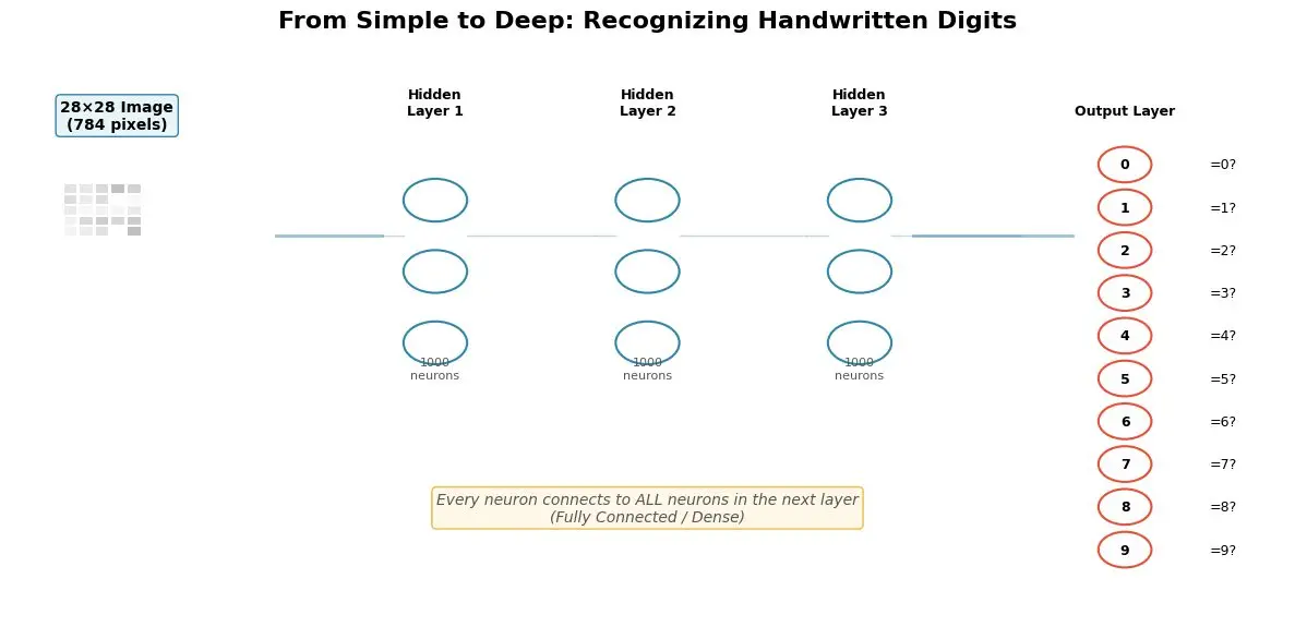
In a fully connected network, every neuron in one layer connects to every neuron in the next layer. If the first hidden layer has 1,000 neurons, and the input has 784 values, that is 784,000 weights just in the first layer!

The math does not change. We still use the chain rule. We still propagate the error backward. We just do it with vectors and matrices instead of single numbers. The book shows this beautifully using matrix notation:

z₁ = W₁ᵀx + b₁ → a₁ = sigmoid(z₁)

z₂ = W₂ᵀa₁ + b₂ → a₂ = sigmoid(z₂)

...and so on...

The algorithm scales to any number of layers and any number of neurons. That is its superpower.

9. What Is the Network Actually Learning?

Here is a question that confused scientists for decades: What exactly is happening inside those hidden layers?

The answer, as Rumelhart, Hinton, and Williams discovered, is that the network is learning representations. It is discovering its own features.

Imagine you want to separate circles from triangles in a picture. If you only look at the raw x and y coordinates, you cannot draw a straight line to separate them. You need a new feature — maybe something like x1 × x2 — to make the separation possible.

Old algorithms forced humans to design these features by hand. But a neural network with hidden layers figures them out automatically. The hidden neurons learn to detect edges, curves, corners, and patterns that are useful for the task. As the book says, "internal 'hidden' units come to represent important features of the task domain."

This is why their famous paper was titled "Learning Representations by Back-propagating Errors." The errors do not just fix the weights — they create understanding inside the hidden layers.

10. The Random Start: Breaking Symmetry

There is one more secret we must mention. When we first create the network, all the weights are random. Why random?

Imagine if all weights started at exactly the same number — say, zero. Every hidden neuron would compute the exact same thing. They would all learn the exact same feature. You could have 1,000 neurons, but they would act like one neuron. That is a waste.

By starting with small random weights (sampled from a Gaussian distribution, as the book explains), we break the symmetry. Each neuron begins its journey from a different starting point, so each one learns something different. One neuron might learn to detect vertical lines, another horizontal lines, another curves. Together, they build a rich understanding of the world.

11. The Sigmoid: Why This Shape?

You might wonder: why did we choose the sigmoid function? Why not something else?

The book includes a "Mathematical Coda" that proves a beautiful fact: the derivative of the sigmoid can be written using the sigmoid itself:

d/dz sigmoid(z) = sigmoid(z) × (1 - sigmoid(z))

This means if we already calculated yhat = sigmoid(z), we can find the slope using just yhat. We do not need to recalculate the exponential function. This saves enormous amounts of computing power.

But there is a deeper reason: the sigmoid is smooth and differentiable everywhere. In the 1970s, researchers used binary threshold neurons — neurons that jumped directly from 0 to 1 at a certain point. These jumps are not differentiable (you cannot find a slope at a cliff), so backpropagation cannot work through them.

The sigmoid was one of the key advances that made backpropagation possible. It turned sharp cliffs into smooth hills, allowing the algorithm to slide down toward the correct answer.

12. Python From Scratch: Building Our Own Brain

Now let us build a complete neural network using only Python and NumPy — no TensorFlow, no PyTorch, no black boxes. We will teach it to solve the XOR problem, a classic puzzle that a single-layer network cannot solve.

The XOR Problem

Input 1	Input 2	Output
0	0	0
0	1	1
1	0	1
1	1	0

You cannot draw a straight line to separate the 0s from the 1s. You need a hidden layer to learn a curved boundary.

The Code

```

import numpy as np

class SimpleNeuralNetwork:

def __init__(self, input_size, hidden_size, output_size):

# Step 1: Random weights (breaking symmetry!)

self.W1 = np.random.randn(input_size, hidden_size) * 0.5

self.b1 = np.random.randn(1, hidden_size) * 0.5

self.W2 = np.random.randn(hidden_size, output_size) * 0.5

self.b2 = np.random.randn(1, output_size) * 0.5

def sigmoid(self, z):

return 1 / (1 + np.exp(-z))

def sigmoid_derivative(self, a):

# Beautiful shortcut: derivative uses the output itself

return a * (1 - a)

def forward(self, X):

# Forward pass: making a guess

self.z1 = np.dot(X, self.W1) + self.b1

self.a1 = self.sigmoid(self.z1)

self.z2 = np.dot(self.a1, self.W2) + self.b2

self.yhat = self.sigmoid(self.z2)

return self.yhat

def backward(self, X, y, learning_rate=0.5):

m = X.shape[0]

# Calculate error

error = self.yhat - y

loss = np.mean(error ** 2)

# Output layer gradients (chain rule!)

dL_dyhat = 2 * error / m

dyhat_dz2 = self.sigmoid_derivative(self.yhat)

delta2 = dL_dyhat * dyhat_dz2

dW2 = np.dot(self.a1.T, delta2)

db2 = np.sum(delta2, axis=0, keepdims=True)

# Hidden layer gradients (backpropagating the blame!)

delta1 = np.dot(delta2, self.W2.T) * self.sigmoid_derivative(self.a1)

dW1 = np.dot(X.T, delta1)

db1 = np.sum(delta1, axis=0, keepdims=True)

# Update weights (gradient descent)

self.W2 -= learning_rate * dW2

self.b2 -= learning_rate * db2

self.W1 -= learning_rate * dW1

self.b1 -= learning_rate * db1

return loss

def train(self, X, y, epochs=10000, learning_rate=0.5):

for i in range(epochs):

self.forward(X)

loss = self.backward(X, y, learning_rate)

if i % 1000 == 0:

print(f"Epoch {i}, Loss: {loss:.6f}")

return self.loss_history

# The XOR data

X = np.array([[0, 0], [0, 1], [1, 0], [1, 1]])

y = np.array([[0], [1], [1], [0]])

# Create and train

nn = SimpleNeuralNetwork(2, 2, 1)

nn.train(X, y, epochs=10000, learning_rate=0.5)

# Test

print("Final predictions:")

print(nn.forward(X).round(3))

```

What Happens When We Run It?

When we start, the network knows nothing. Its predictions are random — around 0.5 to 0.6 for every input.

But after training, something magical happens:

Final predictions:

[[0.031] ← Close to 0!

[0.973] ← Close to 1!

[0.028]] ← Close to 0!

The network learned the XOR pattern! It discovered, inside its hidden neurons, a way to draw a curved boundary that separates the answers.

13. Watching the Network Learn

Let us look at two pictures that show what is happening inside the network.

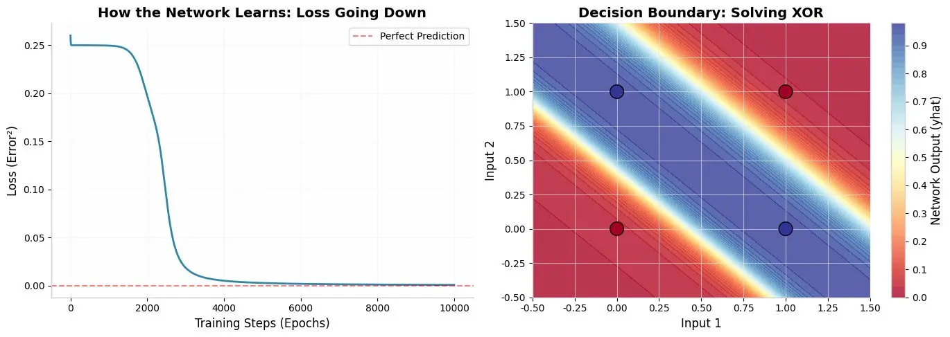
Left Picture: The Loss Curve

At the beginning (Epoch 0), the loss is high — around 0.26. The network is making big mistakes. But slowly, as backpropagation adjusts the weights, the loss drops. By Epoch 3000, it falls off a cliff. By Epoch 10,000, it is nearly zero. This is the network "getting it."

Right Picture: The Decision Boundary

The background shows what the network predicts for every possible combination of inputs. Red means "predict 0," blue means "predict 1." The four big dots are our training data. The network learned to draw a diagonal boundary that perfectly separates the red dots from the blue dots. A straight line could never do this. The hidden layer gave the network the power to learn a curve.

14. The Big Picture: Why This Changed Everything

Before backpropagation, machine learning algorithms needed humans to be very clever. Humans had to design features, choose kernels, and engineer solutions by hand. It was like building a car by carving every part manually.

Backpropagation changed the rules. It said: Give the network the raw data, give it the correct answers, and it will figure out the rest. The network will design its own features. It will find its own patterns. It will build its own internal world.

This is why deep learning exploded. Today, networks have hundreds of layers and billions of weights. They translate languages, generate art, drive cars, and discover new medicines. But underneath all that complexity, the engine is still the same four steps that Rumelhart, Hinton, and Williams published in their three-page paper in Nature:

Forward pass: Make a guess.
Calculate loss: Measure the mistake.
Backward pass: Send the blame back using the chain rule.
Update weights: Turn the knobs in the right direction.

Repeat thousands of times, and magic happens.

15. Reference

Anil Ananthaswamy, Why Machines Learn: The Elegant Math Behind Modern AI (2024)