The Algorithm That Ended the "Neural Networks Are Dead" Myth

Machine-Learning tutorial · PySpark.in

How Backpropagation Brought Neural Networks Back to Life

"This was before the Minsky and Papert proof about [neural networks] not working for XOR," said Anil Ananthaswamy to Geoffrey Hinton.

"Yes," Hinton replied, "but I can't let it go [about] it not working for XOR. I reserve the right to complain about that."

— From "Why Machines Learn" by Anil Ananthaswamy, Chapter 10

​The Setup: A Scientific Drama in Three Acts

Imagine you are a young scientist in the 1960s. You believe that machines can learn like brains do. You are excited about neural networks — computer programs that mimic how neurons in the brain connect and fire together.

Then, two famous professors — Marvin Minsky and Seymour Papert — publish a book called "Perceptrons" in 1969. They prove something shocking:

A single-layer neural network cannot solve the XOR problem.

This sounds simple, but it was devastating. The AI community took it to mean: "Neural networks are useless." Funding dried up. Research stopped. The field entered what people call the "AI Winter."

But here is the thing Minsky and Papert did NOT prove:

They only proved that simple, single-layer networks fail. They said nothing about multi-layer networks with hidden neurons.

It was like saying: "A bicycle cannot climb a mountain, therefore no vehicle can climb a mountain." They ignored the possibility of cars, trucks, or helicopters.

One young man — Geoffrey Hinton — saw through this. And he would spend the next 20 years proving the world wrong.

​ Meet Geoffrey Hinton: The Man Who Would Not Give Up

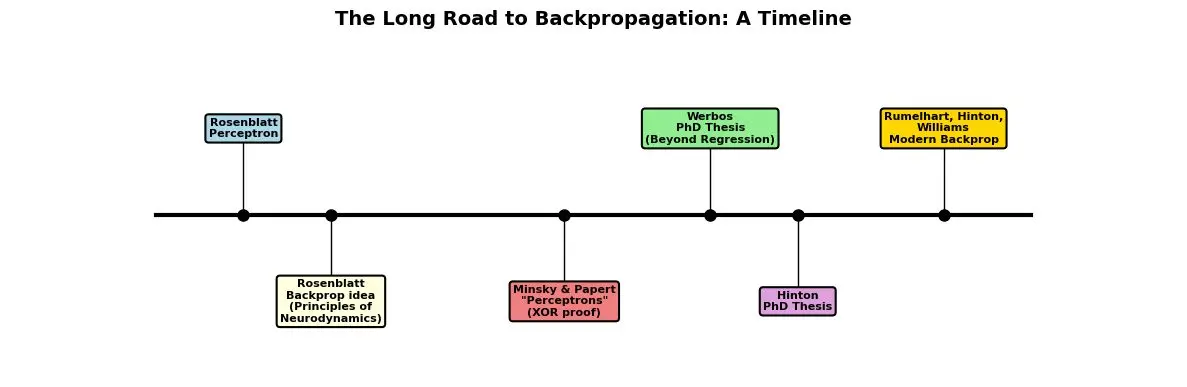
Figure 1: The long road to backpropagation. Good ideas never truly die — they just wait for the right person to pick them up.

Geoffrey Hinton became interested in neural networks as a teenager in high school in the United Kingdom. A mathematician friend was wondering how memories are stored in the brain. Scientists had just figured out how to make 3D holograms.

"He got interested in the idea that the brain might be like a hologram in that memory is not localized," Hinton recalled.

While his friend explored memory storage, Hinton became interested in how brains learn. He wanted to understand the mind.

​The Academic Journey

Hinton studied physics and physiology at university, hoping to learn how the brain works. But all they taught was how electrical signals travel along neurons — not how thinking happens.

Disappointed, he turned to philosophy. He thought philosophers might have answers. They didn't.

"They didn't have the Feynman concept of understanding the mind — that you need to figure out how to build one to understand it."

He even tried experimental psychology, but found it unsatisfying:

"What they did was design experiments to distinguish between two hypotheses, both of which were obviously hopeless. That didn't satisfy me."

Frustrated, Hinton did some carpentry and read books. One book changed everything: Donald Hebb's "The Organization of Behavior."

In 1972, Hinton joined the University of Edinburgh to work on his PhD. His advisor, Christopher Longuet-Higgins, had moved from believing in neural networks to believing in symbolic AI — the idea that intelligence comes from following logical rules.

"He spent the whole time trying to get me to switch," Hinton said.

But Hinton refused. He negotiated a deal: six months to work on neural networks. If he produced nothing good, he would switch to symbolic AI.

"And after six months, I said, 'Yeah, well, I haven't produced anything good. But I think I'm going to be able to, so I need another six months.' I kept going like that."

Hinton finished his PhD. His work involved neural networks, but as he admitted: "they weren't learning."

Still, he was convinced that multi-layer neural networks could one day be made to learn.

​ The XOR Problem: Why One Line Is Never Enough

Let us understand what Minsky and Papert proved, and why it mattered.

​What is XOR?

XOR stands for "Exclusive OR." It is a simple logic puzzle:

The rule is: Output is 1 when the inputs are DIFFERENT. Output is 0 when they are the SAME.

​The Problem: No Single Line Works

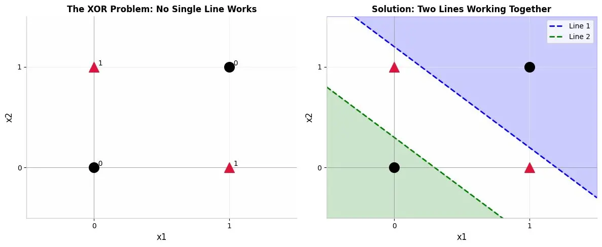
Figure 2: Left — The XOR problem. You cannot draw one straight line that separates the black circles (output 0) from the red triangles (output 1). Right — But TWO lines working together CAN solve it!

Look at the left picture above. The black circles are at positions (0,0) and (1,1). The red triangles are at (0,1) and (1,0).

Can you draw ONE straight line that separates all circles from all triangles?

Try it. You cannot. No matter how you draw the line, at least one point will be on the wrong side.

This is what Minsky and Papert proved mathematically: A single neuron (which draws one line) cannot solve XOR.

​But What About TWO Lines?

Now look at the right picture. If you draw two lines, you CAN separate the points:

• One line separates the top-left from the bottom-right
• Another line separates the top-right from the bottom-left
• The region between the two lines contains the red triangles
• The regions outside contain the black circles

This is the key insight: You need MULTIPLE lines, combined together, to solve XOR.

And multiple lines require multiple layers of neurons — a hidden layer!

​ The Missing Piece: How to Train Multiple Layers

Here is the real problem that stopped everyone for 20 years:

Even if you build a multi-layer network, how do you train it?

In a single-layer network, training is easy:

1. Make a prediction
2. See how wrong you are
3. Adjust the weights

But in a multi-layer network:

1. The input goes through hidden neurons
2. The hidden neurons feed the output neuron
3. If the final answer is wrong, which weight should you change?

Should you blame the output neuron's weights? Or the hidden neuron's weights? Or both? And by how much?

This was the puzzle that Frank Rosenblatt (inventor of the Perceptron) had glimpsed, Paul Werbos had partially solved, and Geoffrey Hinton, David Rumelhart, and Ronald Williams would finally crack in the early 1980s.

​ The Forgotten Prophet: Frank Rosenblatt

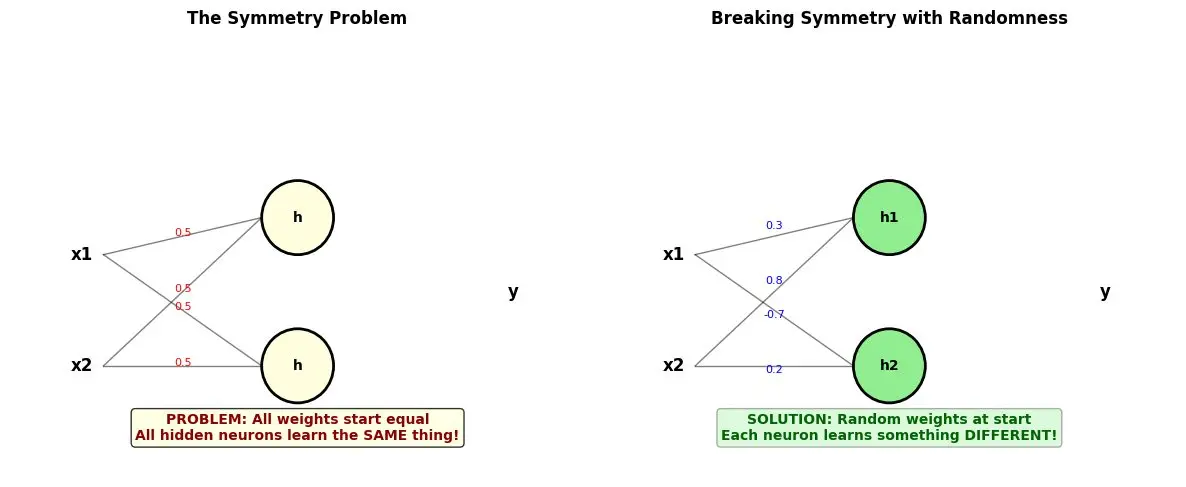
Figure 3: Left — If all weights start equal, all hidden neurons learn the same thing. Right — Random initialization breaks symmetry, letting each neuron learn something different.

Here is a surprising fact: Frank Rosenblatt, the inventor of the Perceptron, had already thought about training multi-layer networks!

In his 1961 book "Principles of Neurodynamics," Rosenblatt described a "back-propagating error correction procedure." He wrote:

"The procedure to be described here is called the 'back-propagating error correction procedure' since it takes its cue from the error of the R-units, propagating corrections back towards the sensory end of the network."

Rosenblatt understood the basic idea: If the output is wrong, send the error backward through the network to fix the weights.

But there was a catch. Rosenblatt's network had predetermined weights for the first layer. Only the last layer was trainable. He wrote:

"It would seem that considerable improvement in performance might be obtained if the values of the [first layer] connections could somehow be optimized by a learning process, rather than accepting the arbitrary or pre-designed network."

He had the right intuition but couldn't make it work fully.

​The Symmetry Problem

Rosenblatt also identified another problem. Imagine a three-layer network where all weights start at zero:

• Every hidden neuron receives the same input
• Every hidden neuron produces the same output
• Every hidden neuron gets updated the same way
• Result: All hidden neurons learn the exact same thing!

You might as well have just one hidden neuron. This is called the symmetry problem.

Rosenblatt suggested using randomness — a stochastic process — to break this symmetry. Hinton tried this idea but found it didn't work well.

The elegant solution would come later, from an unexpected direction.

​ Hinton's Journey to America

After finishing his PhD in 1977, Hinton found no support in the UK. The academic world had turned against neural networks.

"I was so fed up with the fact that nobody else seemed to believe in neural nets that I abandoned academia and went and taught in a free school."

He taught math to inner-city kids at the White Lion Street Free School in London. The school had no paper, so he used the backs of his thesis drafts to teach.

After six months, he wanted back into academia. He could barely get interviews. Finally, an academic at Sussex suggested:

"Make reduction photocopies of your thesis and mail them to everyone you had heard of in the United States. Because that's where AI was."

David Rumelhart at UC San Diego read Hinton's thesis and offered him a postdoc.

For Hinton, America was a revelation. In Britain, neural networks were heresy. In the US:

"I'd never been anywhere where neural nets weren't considered to be nonsense."

It was the early 1980s. The contours of what would become the backpropagation algorithm were becoming clear.

​The Math That Makes It Work: Gradient Descent and the Chain Rule

Before we understand backpropagation, we need two mathematical tools. Don't worry — they are simpler than they sound!

​Tool 1: Gradient Descent — Walking Downhill

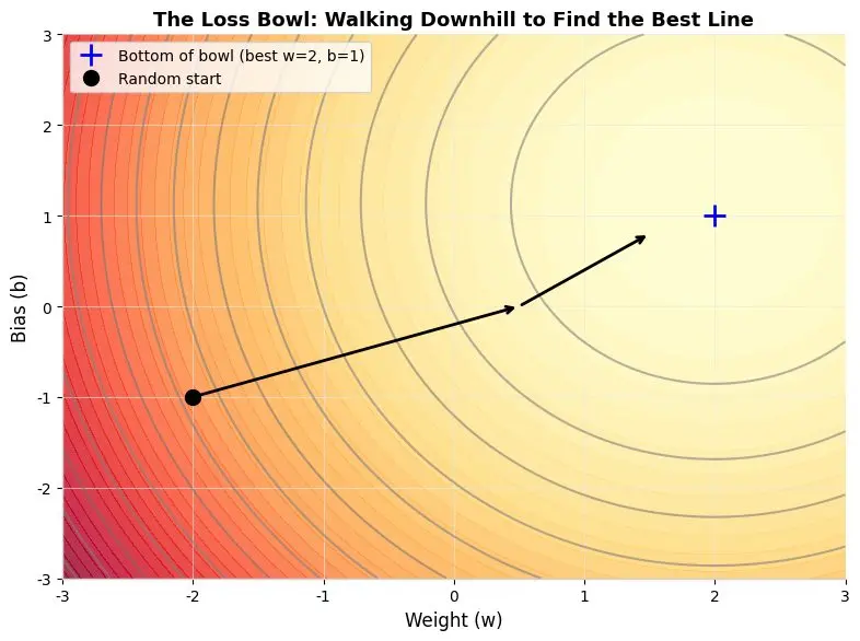
Figure 4: The loss bowl. Imagine you are on a hillside and want to reach the valley bottom. You look around, find the steepest downhill direction, and take a small step. Repeat!

Imagine you are on a mountain and want to reach the lowest valley. You cannot see the whole mountain — it is foggy. What do you do?

1. Feel the ground around your feet. Which direction goes downhill?
2. Take a small step in that direction.
3. Repeat until you reach the bottom.

This is gradient descent. In neural networks:

• The "mountain" is the loss function — a measure of how wrong your predictions are
• The "valley bottom" is where the loss is smallest — where predictions are best
• The "direction" is the gradient — calculated using calculus

​Tool 2: The Chain Rule — Passing the Blame Backward

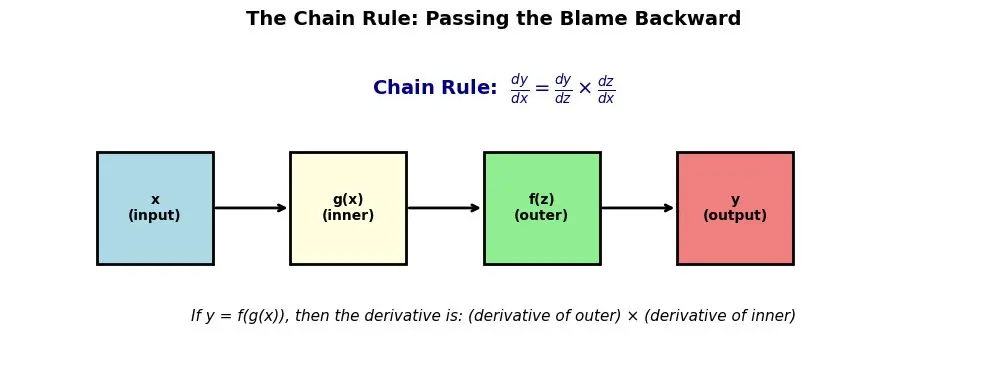
Figure 5: The chain rule. If y depends on z, and z depends on x, then the derivative of y with respect to x is the product of the two derivatives. This lets us "pass the blame" backward through the network.

The chain rule from calculus says:

If something depends on something, which depends on something else, you can chain the derivatives together.

For example, if:

• y = f(z) (output depends on hidden value)
• z = g(x) (hidden value depends on input)

Then:

dy/dx = dy/dz × dz/dx

This is the mathematical engine of backpropagation. It lets us ask:

"How much does the final error depend on this specific weight deep in the network?"

By chaining derivatives from the output all the way back to the input, we can calculate exactly how to adjust every weight.

​Backpropagation: The Full Story

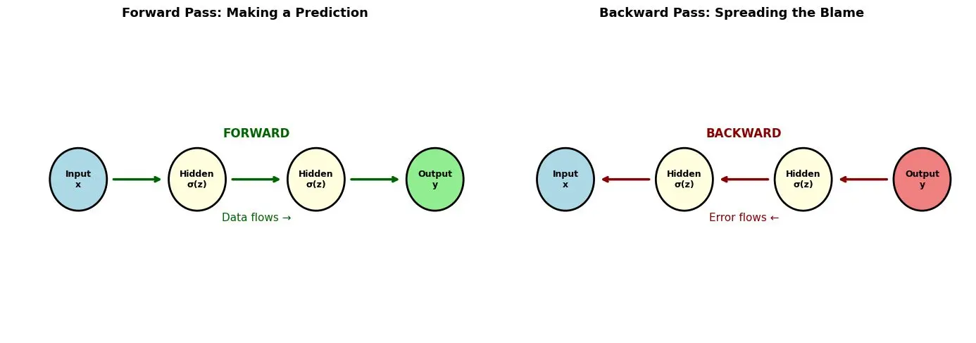
Figure 6: Forward pass (green): Data flows from input to output, making a prediction. Backward pass (red): Error flows from output back to input, updating weights.

Backpropagation has two phases, repeated thousands of times:

​Phase 1: Forward Pass — Make a Prediction

1. Input data enters the network
2. Each neuron computes: z = (weight × input) + bias
3. Apply activation function: a = sigmoid(z)
4. Pass output to next layer
5. Final layer produces prediction

​Phase 2: Backward Pass — Spread the Blame

1. Compare prediction to true answer → calculate error
2. Ask: "How much did each output weight contribute to this error?"
3. Use chain rule to ask: "How much did each hidden weight contribute?"
4. Continue backward to input layer
5. Update ALL weights by a small amount in the direction that reduces error

This is why it is called back-propagation — the error signal propagates backward through the network.

​Python Example 1: A Single Neuron Learns a Straight Line

Let us start simple. Here is a single neuron learning to fit a straight line — no libraries, pure Python!

```

# ============================================

# EXAMPLE 1: A Single Neuron Learns a Straight Line

# No libraries needed - pure Python!

# ============================================

# Training data: x values and their corresponding y values

# The true relationship is: y = 2*x + 1 (but the neuron doesn't know this!)

training_data = [

(-2, -3.1), (-1.5, -2.0), (-1, -0.9), (-0.5, 0.1),

(0, 1.0), (0.5, 1.9), (1, 3.1), (1.5, 4.0),

(2, 5.1), (2.5, 5.9)

]

# Step 1: Start with random guesses for weight and bias

weight = 0.0 # Our guess for the slope

bias = 0.0 # Our guess for the offset

learning_rate = 0.01

# Step 2: Training loop - repeat many times

for epoch in range(1000):

total_loss = 0

for x, y_true in training_data:

# FORWARD PASS: Make a prediction

y_predicted = weight * x + bias

# Calculate error

error = y_true - y_predicted

total_loss += error ** 2

# BACKWARD PASS: Calculate how to fix weight and bias

# Using the chain rule (simplified):

gradient_weight = -2 * x * error

gradient_bias = -2 * error

# UPDATE: Move a small step in the opposite direction

weight = weight - learning_rate * gradient_weight

bias = bias - learning_rate * gradient_bias

# Print progress every 100 epochs

if epoch % 100 == 0:

avg_loss = total_loss / len(training_data)

print(f"Epoch {epoch:4d}: weight={weight:6.3f}, bias={bias:6.3f}, loss={avg_loss:.4f}")

print(f"\nFINAL: Learned: y = {weight:.3f}*x + {bias:.3f}")

print(f" True: y = 2.000*x + 1.000")

```

Output:

Epoch 0: weight= 0.761, bias= 0.260, loss=7.6819

Epoch 100: weight= 1.997, bias= 1.009, loss=0.0074

...

FINAL: Learned: y = 1.997*x + 1.009

True: y = 2.000*x + 1.000

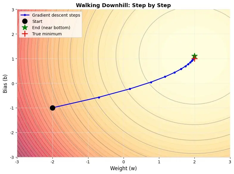
Figure 7: The neuron starts at a random point and walks downhill step by step until it finds the best weight and bias values.

The neuron starts with weight=0 and bias=0 — a terrible guess. But by repeatedly calculating gradients and taking small steps, it converges to weight≈2 and bias≈1 — the correct answer!

​Python Example 2: A Neuron Learns the AND Gate

Now let us add a non-linear activation function — the sigmoid — and learn a simple logic gate.

```

import math

# AND gate truth table

training_data = [

([0, 0], 0),

([0, 1], 0),

([1, 0], 0),

([1, 1], 1),

]

def sigmoid(z):

return 1.0 / (1.0 + math.exp(-z))

def sigmoid_derivative(a):

return a * (1 - a)

# Random weights

w1, w2, bias = 0.1, -0.2, 0.0

learning_rate = 0.1

for epoch in range(5000):

for (x1, x2), y_true in training_data:

# Forward pass

z = w1 * x1 + w2 * x2 + bias

y_pred = sigmoid(z)

error = y_true - y_pred

# Backward pass (chain rule)

d_loss_d_y = -2 * error

d_y_d_z = sigmoid_derivative(y_pred)

grad_w1 = d_loss_d_y * d_y_d_z * x1

grad_w2 = d_loss_d_y * d_y_d_z * x2

grad_b = d_loss_d_y * d_y_d_z

# Update

w1 -= learning_rate * grad_w1

w2 -= learning_rate * grad_w2

bias -= learning_rate * grad_b

# Test

for (x1, x2), y_true in training_data:

z = w1 * x1 + w2 * x2 + bias

y_pred = sigmoid(z)

print(f"x1={x1}, x2={x2}: predicted={y_pred:.4f}, true={y_true}")

```

Output:

x1=0, x2=0: predicted=0.0002, true=0

x1=0, x2=1: predicted=0.0556, true=0

x1=1, x2=0: predicted=0.0556, true=0

x1=1, x2=1: predicted=0.9340, true=1

The neuron learned to output values close to 0 for (0,0), (0,1), (1,0) and close to 1 for (1,1). It learned the AND gate!

​Python Example 3: The Full Neural Network Solves XOR!

Now for the main event. Here is a complete two-layer neural network that solves the "impossible" XOR problem — implemented from scratch in pure Python!

PythonCopy

```

import math

import random

# XOR truth table

training_data = [

([0, 0], 0),

([0, 1], 1),

([1, 0], 1),

([1, 1], 0),

]

def sigmoid(z):

return 1.0 / (1.0 + math.exp(-z))

def sigmoid_derivative(a):

return a * (1 - a)

# Network: 2 inputs → 2 hidden → 1 output

# RANDOM initialization (breaks symmetry!)

random.seed(42)

# Input to hidden weights

w_i1_h1 = random.uniform(-1, 1)

w_i2_h1 = random.uniform(-1, 1)

b_h1 = random.uniform(-1, 1)

w_i1_h2 = random.uniform(-1, 1)

w_i2_h2 = random.uniform(-1, 1)

b_h2 = random.uniform(-1, 1)

# Hidden to output weights

w_h1_o = random.uniform(-1, 1)

w_h2_o = random.uniform(-1, 1)

b_o = random.uniform(-1, 1)

learning_rate = 0.5

# Training

for epoch in range(10000):

total_loss = 0

for (x1, x2), y_true in training_data:

# ===== FORWARD PASS =====

z_h1 = w_i1_h1 * x1 + w_i2_h1 * x2 + b_h1

a_h1 = sigmoid(z_h1)

z_h2 = w_i1_h2 * x1 + w_i2_h2 * x2 + b_h2

a_h2 = sigmoid(z_h2)

z_o = w_h1_o * a_h1 + w_h2_o * a_h2 + b_o

y_pred = sigmoid(z_o)

error = y_true - y_pred

total_loss += error ** 2

# ===== BACKWARD PASS (Chain Rule!) =====

d_loss_d_y = -2 * error

d_y_d_zo = sigmoid_derivative(y_pred)

# Output layer gradients

grad_w_h1_o = d_loss_d_y * d_y_d_zo * a_h1

grad_w_h2_o = d_loss_d_y * d_y_d_zo * a_h2

grad_b_o = d_loss_d_y * d_y_d_zo

# Hidden layer 1 gradients (chain rule through output!)

d_loss_d_ah1 = d_loss_d_y * d_y_d_zo * w_h1_o

d_ah1_d_zh1 = sigmoid_derivative(a_h1)

grad_w_i1_h1 = d_loss_d_ah1 * d_ah1_d_zh1 * x1

grad_w_i2_h1 = d_loss_d_ah1 * d_ah1_d_zh1 * x2

grad_b_h1 = d_loss_d_ah1 * d_ah1_d_zh1

# Hidden layer 2 gradients

d_loss_d_ah2 = d_loss_d_y * d_y_d_zo * w_h2_o

d_ah2_d_zh2 = sigmoid_derivative(a_h2)

grad_w_i1_h2 = d_loss_d_ah2 * d_ah2_d_zh2 * x1

grad_w_i2_h2 = d_loss_d_ah2 * d_ah2_d_zh2 * x2

grad_b_h2 = d_loss_d_ah2 * d_ah2_d_zh2

# ===== UPDATE ALL WEIGHTS =====

w_h1_o -= learning_rate * grad_w_h1_o

w_h2_o -= learning_rate * grad_w_h2_o

b_o -= learning_rate * grad_b_o

w_i1_h1 -= learning_rate * grad_w_i1_h1

w_i2_h1 -= learning_rate * grad_w_i2_h1

b_h1 -= learning_rate * grad_b_h1

w_i1_h2 -= learning_rate * grad_w_i1_h2

w_i2_h2 -= learning_rate * grad_w_i2_h2

b_h2 -= learning_rate * grad_b_h2

if epoch % 1000 == 0:

print(f"Epoch {epoch}: loss = {total_loss:.6f}")

# Test

print("\nFinal Results:")

for (x1, x2), y_true in training_data:

z_h1 = w_i1_h1 * x1 + w_i2_h1 * x2 + b_h1

a_h1 = sigmoid(z_h1)

z_h2 = w_i1_h2 * x1 + w_i2_h2 * x2 + b_h2

a_h2 = sigmoid(z_h2)

z_o = w_h1_o * a_h1 + w_h2_o * a_h2 + b_o

y_pred = sigmoid(z_o)

print(f"x1={x1}, x2={x2}: predicted={y_pred:.4f}, true={y_true}")

```

Output:

Epoch 0: loss = 1.119092

Epoch 1000: loss = 0.011399

Epoch 2000: loss = 0.003668

...

Epoch 9000: loss = 0.000598

Final Results:

x1=0, x2=0: predicted=0.0116, true=0 ✓

x1=0, x2=1: predicted=0.9868, true=1 ✓

x1=1, x2=0: predicted=0.9892, true=1 ✓

x1=1, x2=1: predicted=0.0103, true=0 ✓

 SUCCESS! The network learned XOR perfectly!

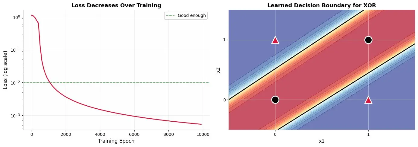
Figure 8: Left — The loss decreases rapidly during training. Right — The learned decision boundary. The network found a curved region (the band between two lines) that perfectly separates the XOR points!

​How the Network Solves XOR: Step by Step

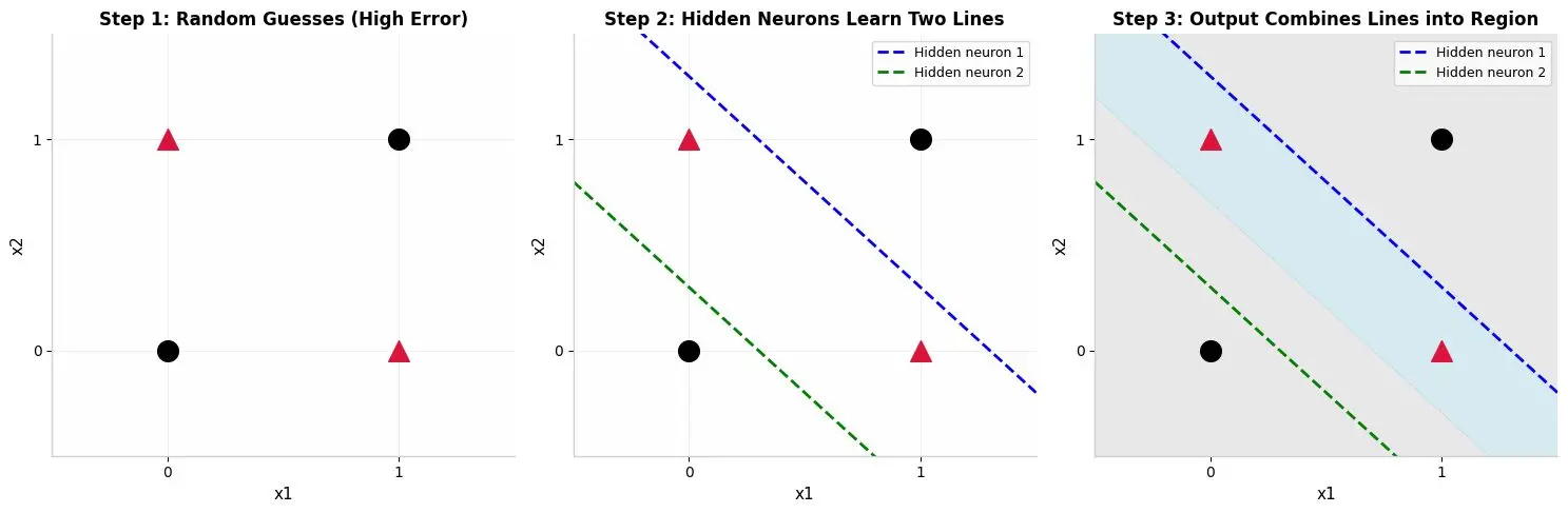
Figure 9: How the network learns XOR over time. Step 1 — Random weights give random predictions. Step 2 — Hidden neurons each learn a line. Step 3 — The output neuron combines the lines into a region that separates the points correctly.

Let us understand what happened inside the network:

​Hidden Neuron 1 learned one line:

z = 6.52*x1 + (-6.69)*x2 + (-3.50)

This line separates some points from others.

​Hidden Neuron 2 learned another line:

z = 6.19*x1 + (-6.01)*x2 + 3.01

This line separates points differently.

​The Output Neuron learned to COMBINE:

z = 10.20*h1 + (-10.00)*h2 + 4.79

The output neuron says: "If h1 is active AND h2 is NOT active, output 1. Otherwise, output 0."

This is exactly the XOR logic! The network learned to:

1. Transform the input space using two lines
2. Combine the transformed features to create a non-linear decision boundary

​The Non-Convex Problem: Hills and Valleys

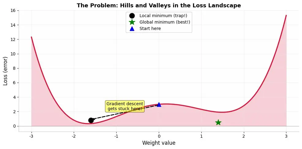
Figure 10: The loss landscape for multi-layer networks is not a simple bowl. It has many hills and valleys. Gradient descent can get stuck in a local minimum — a valley that is not the lowest point.

Here is a problem we have not discussed yet. In a single neuron, the loss landscape is a simple bowl — one smooth valley. Gradient descent is guaranteed to find the bottom.

But in multi-layer networks, the loss landscape is much more complex:

It has many hills and valleys — what mathematicians call a non-convex function.

This means gradient descent might:

• Get stuck in a local minimum (a valley that is not the deepest)
• Fall off a plateau (a flat area where nothing seems to improve)
• Oscillate between steep walls

Minsky and Oliver Selfridge had studied this in 1961. They called it the "mesa phenomenon" — flat elevated regions where small changes don't help.

This was one reason Minsky became pessimistic about neural networks. But here is what he missed:

In practice, local minima are often "good enough." And modern techniques (momentum, adaptive learning rates, better initialization) help avoid the worst traps.

​The Wider History: Many Hands, One Idea

Backpropagation was not invented in one place by one person. It emerged from multiple fields over decades:

Paul Werbos came closest in 1974. But his thesis was:

• Not publicized much
• Not aimed at neural network researchers
• Written for behavioral scientists

It took Rumelhart, Hinton, and Williams in the early 1980s to:

• Present backpropagation clearly
• Show it could solve real problems like XOR
• Demonstrate it could train practical multi-layer networks

This version gave deep neural networks the boost they needed to survive the AI winter.

​ Why This Matters: The Foundation of Modern AI

Everything you use today — ChatGPT, image recognition, voice assistants, self-driving cars — traces back to this algorithm.

Backpropagation is the universal learning engine that makes deep neural networks possible. Without it:

• Networks could only have one layer
• They could only solve simple, linear problems
• AI would still be stuck in the 1960s

With backpropagation:

• Networks can have hundreds of layers
• They can learn complex, non-linear patterns
• They can recognize faces, translate languages, generate art, and more

The "impossible" XOR problem — solved by a tiny network with just 2 hidden neurons — was the proof of concept that opened the door to everything.

​ Summary: Key Takeaways

​ For Beginners: What to Remember

1. A single neuron draws one line. Some problems need more than one line.
2. A hidden layer means multiple neurons working together. Each hidden neuron learns a different "feature" or "line."
3. Backpropagation is like a teacher giving feedback. The teacher looks at the final answer, calculates how wrong it is, then tells every student (neuron) exactly how much they contributed to the mistake.
4. The chain rule is like a game of telephone in reverse. The error message starts at the output and gets passed backward, with each layer adding information about how much it contributed.
5. Random initialization breaks symmetry. If all neurons start the same, they learn the same thing. Randomness makes each neuron unique.
6. Training is just walking downhill. You cannot see the whole mountain, but you can feel which way is down and take a step.

​Book Reference

"Why Machines Learn: The Elegant Math Behind Modern AI"

by Anil Ananthaswamy

Published by Dutton (2024)

More Machine-Learning tutorials

• Introduction to Machine Learning
• Introduction to Deep Learning
• ​A Beginner's Guide to Machine Learning
• The First Artificial Neuron and Learning from Mistakes
• ​Patterns
• ​ Understanding Vectors, the Building Blocks of AI

All tutorials · Try the free PySpark compiler · Practice challenges