One Hidden Layer Is All You Need? The Surprising Story of George Cybenko and the Universal Power of Neural Networks

Machine-Learning tutorial · PySpark.in

Welcome back to our simple-English machine learning series! If you are new here — don't worry. This blog is written for everyone, even if you have never written a single line of code. By the end, you will understand one of the most beautiful ideas in all of machine learning.

1. The Rock Star Professor Who Became a Villain (By Mistake)

In 2017, a professor named George Cybenko taught a summer school on deep learning in Bilbao, Spain. Nearly 1,300 students came. About 400 attended his class. During breaks, students ran up to him asking for selfies.

Cybenko felt like a rock star.

But later, he read a blog post. The blogger wrote that another famous AI researcher, Li Deng, had joked: "The very theorem that made Cybenko feel like a rock star may have substantially set back the field of deep learning."

Cybenko laughed, but also felt strange. In some circles, people said he was "the guy that delayed deep learning by twenty years."

Why? What did Cybenko do that was so powerful — and so misunderstood?

Let us go back in time and understand the full story, step by step.

2. A Quick History Lesson: Why People Gave Up on Neural Networks

To understand Cybenko, we need to know what happened before him.

1950s–1960s: The Birth of Neural Networks

Two scientists, Frank Rosenblatt and Bernard Widrow, created the first neural networks. These were single-layer networks — meaning the input connected directly to the output. No middle layer. They called these perceptrons.

These simple networks could learn some things. People got very excited.

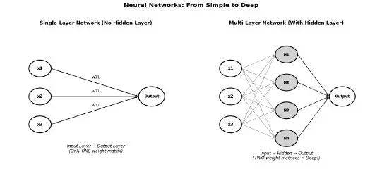
1969: The Book That Killed Hope

Then two other scientists, Marvin Minsky and Seymour Papert, wrote a famous book called Perceptrons. They proved something shocking:

A single-layer neural network cannot solve simple problems.

For example, a single-layer network cannot learn the XOR problem — a very basic "this OR that, but not both" puzzle. It was like discovering your calculator cannot do addition.

Worse, Minsky and Papert hinted (without proof) that maybe multi-layer networks were also useless. This killed almost all research in neural networks. Scientists stopped funding it. Students stopped studying it. This dark time is called the first AI winter.

1981–1982: A Small Light

A scientist named John Hopfield created a new type of network. But it was different — it learned in "one shot," not gradually through training data. It did not bring back the old idea of multi-layer training.

1986: The Comeback

Then, in 1986, three researchers — David Rumelhart, Geoffrey Hinton, and Ronald Williams — published a paper in the famous journal Nature. They showed a training method called backpropagation. This method could finally train multi-layer neural networks.

Deep learning was back on track. Wheels were turning again.

And then — in 1989 — Cybenko published his paper.

3. What Did Cybenko Actually Prove?

Cybenko was a mathematician. He studied signal processing. He saw that people were training multi-layer networks, but no one really understood what these networks could do. He asked a simple question:

"What can a single-hidden-layer network do?"

His answer became one of the most famous theorems in machine learning:

The Universal Approximation Theorem

A neural network with just ONE hidden layer, if it has enough neurons, can approximate ANY function.

Let us break this down in simple words.

What is a "Function"?

A function is just a machine that takes an input and gives an output.

Input = temperature, Output = "will it rain?" → function
Input = your photo, Output = "is this a cat?" → function
Input = words you type, Output = next word to suggest → function

Every machine learning problem is secretly a function. Training a neural network means: find the function that best matches the real world.

What Does "Approximate" Mean?

"Approximate" means "get very close to." Not perfect, but close enough.

Think of it like drawing a curve with straight lines. If you use only 2 lines, it looks bad. If you use 50 tiny lines, it looks almost exactly like the curve. More lines = better match.

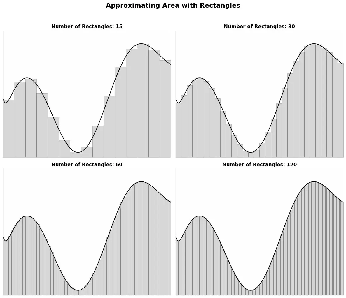
The book shows this idea with rectangles. More rectangles = better area estimate. More neurons = better function estimate.

What Does "Any Function" Mean?

Literally any function. A simple line. A wiggly wave. A speech sound. An image recognizer. A ChatGPT text generator. If you have enough neurons in one hidden layer, the network can get arbitrarily close to matching it.

This was Cybenko's proof. It was mathematical, rigorous, and beautiful.

4. How Does One Hidden Layer Do Magic?

This is the part that amazes people. Let us build the intuition step by step.

Step 1: The Sigmoid — A Bendy Switch

First, we need to understand one special neuron. Cybenko used neurons with a sigmoid activation function.

What is a sigmoid? It is a curve that looks like an "S":

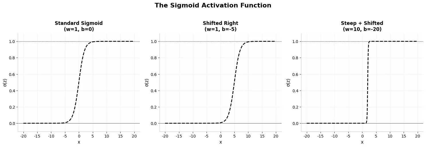
The sigmoid goes smoothly from near 0 to near 1. By changing weight (w) and bias (b), we can shift it left/right and make it steep or gentle.

Here is the math, but do not be scared:

z = w 1x 1 + w 2x 2 + b

y = sigma(z) = (1)/(1 + e^( - z))

In simple words:

Weight (w) controls how steep the S-curve is. Big weight = sharp jump (almost like a step). Small weight = gentle slope.
Bias (b) controls WHERE the jump happens along the x-axis. Change bias = shift left or right.

Step 2: Two Sigmoids Make a Bump

Now here is the magic trick. Take TWO sigmoid neurons in the hidden layer:

Neuron A: jumps UP at position x=0
Neuron B: jumps UP at position x=10

If you add them with opposite signs (A minus B), what happens?

You get a BUMP! A rectangle-shaped hump that is high between 0 and 10, and flat zero everywhere else.

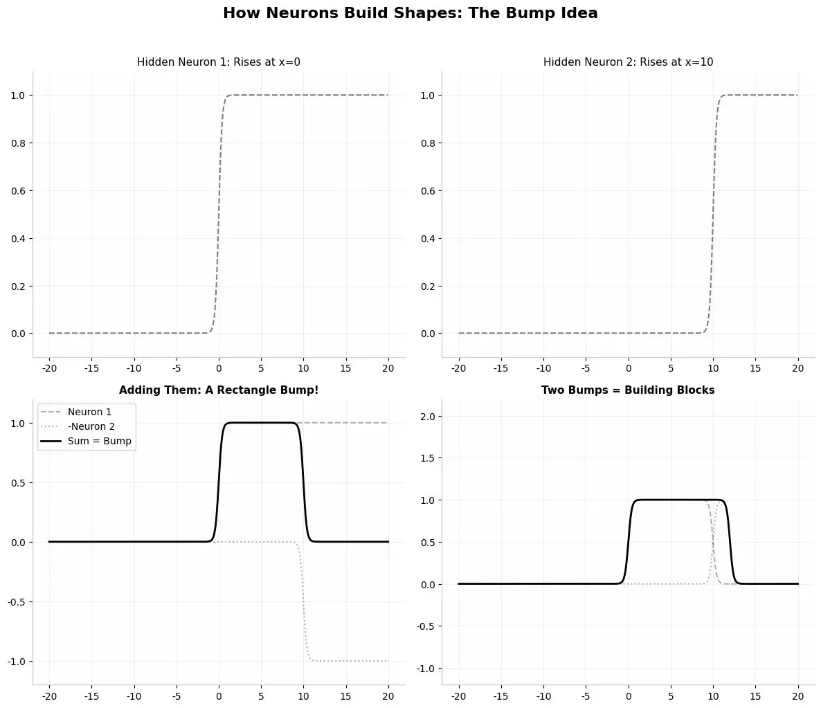
Top left: One neuron rises at x=0. Top right: Another rises at x=10. Bottom left: Subtract them — you get a bump! Bottom right: Two bumps side by side.

Step 3: Many Bumps = Any Shape

If one bump is a building block, then many bumps are like LEGO bricks. Stack them at different heights, different widths, different positions. Add them all together. You can build any shape you want.

This is exactly how a single-hidden-layer network works:

Each hidden neuron creates a sigmoid "step."
Pairs of steps combine into "bumps" (via positive and negative weights).
The output neuron adds all bumps together.
With enough bumps, the final shape matches any target function.

Let us see this in action!

5. Visual Proof: Approximating y = x 2

The book shows this beautiful example. Let us try to approximate the simple parabola

y = x 2

using only sigmoid neurons in one hidden layer.

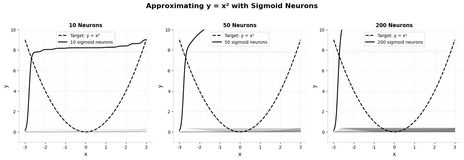
With only 10 neurons, the match is poor. With 50, it improves. With 200, the black line (network output) almost perfectly covers the dashed line (true function).

The lesson: More neurons = more building blocks = better approximation. With enough neurons, you cannot tell the difference between the true function and the network's output.

Now let us try a crazy complicated function — the one from the book:

y = sin(3)/(pix) + cos(3)/(pix) + e - 2pix + |x|

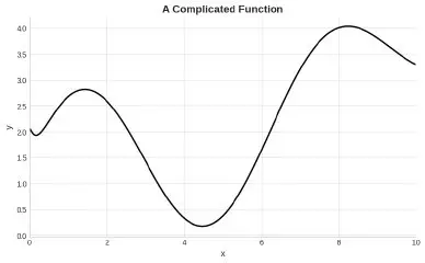
This function wiggles, dips, rises, and curves in complex ways. Can one hidden layer handle it?

Yes! With 300 neurons, the network builds so many tiny bumps that the approximation becomes visually perfect. The solid black line sits exactly on top of the dashed target line.

6. The Big Misunderstanding: Why People Blamed Cybenko

Here is where the story gets ironic.

Cybenko proved: "One hidden layer is enough."

But many researchers misunderstood this. They thought he meant: "You should ONLY use one hidden layer."

So for almost 20 years, people built networks with just one hidden layer. They made that layer very, very wide (thousands of neurons) instead of making the network deep (many layers).

Cybenko himself said: "I didn't say you should use one layer. People concluded that you only need one layer."

Why Did Deep Learning Eventually Win?

Around 2010, researchers realized something important:

"Enough neurons" does not mean "practical number of neurons."

Yes, one hidden layer CAN approximate any function. But it might need millions of neurons to do so. Training millions of neurons in one layer is slow, expensive, and needs impossible amounts of data.

Instead, researchers found that adding more layers (going deep) was far more efficient. A network with 10 layers of 100 neurons each can learn things that would require millions of neurons in a single layer.

This is why deep learning — with many hidden layers — took over. Not because Cybenko was wrong. But because his theorem was about existence (can it be done?), not about efficiency (is it practical?).

7. Functions as Vectors: The Beautiful Math Behind It All

The book takes us on one more mind-bending journey. Cybenko's proof used a powerful idea: functions can be thought of as vectors.

What Does That Mean?

Think of a simple function like y=sin(x) . If we check its value at 11 points (x = 0, 1, 2, ..., 10), we get 11 numbers:

[0.0,0.84,0.91,0.14,−0.76,−0.96,−0.28,0.66,0.99,0.41,−0.54]

This is just a list of numbers. A vector in 11-dimensional space.

Now think of y=cos(x) at the same points:

[1.0,0.54,−0.42,−0.99,−0.65,0.28,0.96,0.75,−0.15,−0.91,−0.84]

Another vector in the same space.

Going to Infinity

Now imagine instead of 11 points, you check infinite points between 0 and 10. Your vector becomes infinitely long. The space becomes infinite-dimensional.

Every function is a point in this infinite-dimensional space.

Cybenko asked: If I take all possible linear combinations of sigmoid functions (from my hidden neurons), do I fill up this entire space? Can I reach every possible function?

His proof by contradiction showed: Yes, you can. The set of sigmoid combinations is "dense" in the function space — meaning you can get arbitrarily close to any function.

This is why the theorem is called universal. It is not about one specific problem. It is about all possible problems.

8. Python From Scratch: Building a Universal Approximator

Let us now build our own tiny universal approximator from scratch — no machine learning libraries! We will manually set weights to approximate a simple function, just to see the idea in action.

```

hide

import numpy as np

import matplotlib.pyplot as plt

# ==============================

# SINGLE HIDDEN LAYER NETWORK

# Built from scratch, no libraries

# ==============================

def sigmoid(z):

"""The S-shaped activation function"""

return 1 / (1 + np.exp(-z))

def hidden_neuron_output(x, weight, bias):

"""One hidden neuron: takes x, applies weight and bias, returns sigmoid"""

z = weight * x + bias

return sigmoid(z)

def network_output(x, hidden_weights, hidden_biases, output_weights):

"""

Full network with ONE hidden layer.

hidden_weights: how steep each hidden neuron's step is

hidden_biases: where each hidden neuron's step happens

output_weights: how much each hidden neuron's output contributes

"""

total = 0

for w_hidden, b_hidden, w_output in zip(hidden_weights, hidden_biases, output_weights):

# Hidden neuron fires

hidden_fire = hidden_neuron_output(x, w_hidden, b_hidden)

# Output neuron adds it with its weight

total += w_output * hidden_fire

return total

# ========================================

# DEMO: Approximating a simple step function

# ========================================

# Create input data

x = np.linspace(-10, 10, 500)

# Target: a step function (0 for x<<0, 1 for x>=0)

target = np.where(x >= 0, 1, 0)

# Build a network with 2 hidden neurons to make ONE bump

# Neuron 1: rises at x = -1 (weight=10, bias=10)

# Neuron 2: rises at x = 1 (weight=10, bias=-10)

hidden_weights = [10, 10] # Both are steep

hidden_biases = [10, -10] # First rises early, second rises late

output_weights = [1, -1] # First adds, second subtracts

# Run the network

prediction = [network_output(xi, hidden_weights, hidden_biases, output_weights)

for xi in x]

# Plot everything

plt.figure(figsize=(10, 6))

# Plot individual hidden neuron outputs

neuron1 = [hidden_neuron_output(xi, 10, 10) for xi in x]

neuron2 = [hidden_neuron_output(xi, 10, -10) for xi in x]

plt.plot(x, neuron1, 'gray', linestyle='--', alpha=0.5, label='Hidden Neuron 1 (rises at x=-1)')

plt.plot(x, neuron2, 'gray', linestyle=':', alpha=0.5, label='Hidden Neuron 2 (rises at x=1)')

plt.plot(x, target, 'black', linestyle='--', linewidth=2, label='Target: Step Function')

plt.plot(x, prediction, 'black', linewidth=2.5, label='Network Output: A Bump!')

plt.title('Building a Bump from Two Sigmoid Neurons', fontsize=14, fontweight='bold')

plt.xlabel('x')

plt.ylabel('Output')

plt.legend()

plt.ylim(-0.2, 1.2)

plt.grid(True, alpha=0.3)

plt.tight_layout()

plt.show()

print("Network created a bump using just 2 hidden neurons!")

```

Output: The code produces a plot showing two gray sigmoid curves and a black "bump" that is their difference. This bump is the network's output — a simple rectangle-like shape built from two smooth S-curves.

Extending to Many Neurons

To approximate a real function like y = x 2 , you would:

Use many more hidden neurons (50, 100, or 300)
Space their "step locations" evenly across the input range
Set their output weights so each contributes the right amount of height
Sum everything at the output neuron

The network learns these weights automatically through backpropagation (which we will cover in the next blog!). But the capacity to represent any function was proven by Cybenko.

9. Why This Matters for You

If you are a beginner, here is what you should take away:

Key Lessons

Table

Idea	Simple Explanation
Universal Approximation	One hidden layer + enough neurons = can learn anything
The Bump Trick	Two sigmoids make a bump; many bumps make any shape
Depth vs Width	One wide layer works in theory, but many layers work better in practice
Cybenko's Legacy	He proved neural networks are powerful; he did NOT say "never go deep"
Functions as Vectors	Any function can be seen as a point in infinite-dimensional space

The Modern Mystery

The book ends Chapter 9 with a fascinating observation. Today's deep networks have billions of neurons and hundreds of layers. By Cybenko's logic, they should suffer from:

The curse of dimensionality (too many parameters)
Overfitting (memorizing instead of learning)

But somehow, they work incredibly well. Scientists are still trying to understand why. The math says one layer is enough. Practice says deep is better. The gap between theory and reality is one of the biggest open questions in machine learning.

10. Summary: The Man Who Did NOT Set Back Deep Learning

George Cybenko proved that neural networks with one hidden layer are universally powerful. This was a mathematical triumph. Some researchers misunderstood it and spent decades building only shallow networks. But the real reason deep learning took until 2010 to explode was not Cybenko's theorem — it was the lack of big data and computing power in the 1990s.

Cybenko himself suspected this. In his 1989 paper, he wrote:

"We suspect quite strongly that the overwhelming majority of approximation problems will require astronomical numbers of terms."

He knew one layer was theoretically enough but practically expensive. Deep networks were the efficient solution waiting for the right hardware and data.

So no — Cybenko did not set back deep learning. He laid the mathematical foundation that made us confident neural networks could work at all.

Reference

Why Machines Learn: The Elegant Math Behind Modern AI

by Anil Ananthaswamy