The Magic Trick That Changed Machine Learning Forever Introduction: A Story from Bell Labs
Machine-Learning tutorial · PySpark.in
In the fall of 1991, a young engineer named Bernhard Boser was waiting to start his new job at the University of California, Berkeley. He had three months to kill. At AT&T Bell Labs in New Jersey, where he was working, he started talking to a Russian mathematician named Vladimir Vapnik. Vapnik was a big name in statistics and machine learning. He had recently moved to the United States.
Vapnik asked Boser to work on an algorithm he had designed back in the 1960s. It was about finding the best possible line (or hyperplane) to separate two groups of data points. Boser implemented it. It worked. But then Vapnik asked him to do something harder: classify data that could NOT be separated by a straight line.
This simple request led to one of the most important inventions in machine learning history: the Support Vector Machine (SVM) and the Kernel Trick. This chapter tells that amazing story.
Part 1: The Perceptron's Problem — Why "Any Line" Is Not Good Enough
What is a Separating Hyperplane?
Imagine you have two groups of points on a piece of paper. One group is circles, the other is triangles. A separating hyperplane is just a fancy name for a line (in 2D) or a plane (in 3D) that divides the two groups.
In simple words: It is a boundary that says, "Everything on this side is a circle, everything on that side is a triangle."
The Perceptron's Limitation
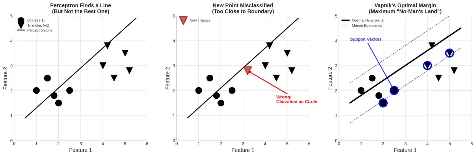
In earlier chapters, we learned about Frank Rosenblatt's perceptron. The perceptron can find a line that separates circles from triangles — IF such a line exists. But here is the problem: if many lines can separate the data, which one should we pick?
The perceptron picks the FIRST line it finds. But that line might be very close to some data points. What happens when a NEW data point comes in, slightly different from the training data? The perceptron might make a mistake.
Look at the picture above:
- Left: The perceptron finds a line. It separates the circles and triangles. Good!
- Middle: A new triangle arrives near the boundary. The perceptron's line classifies it as a circle. Wrong!
- Right: Vapnik's idea — find a line that stays as far as possible from BOTH groups. This is the optimal hyperplane.
The "No-One's-Land" Idea
Vapnik's brilliant idea was to create a "no-one's-land" — a clear path between the two groups. The line should run exactly through the middle of this path. The width of this path is called the margin.
Why is this better? Because if the line is far from both groups, new data points have more room for error. The classifier becomes more robust — it handles new, unseen data better.
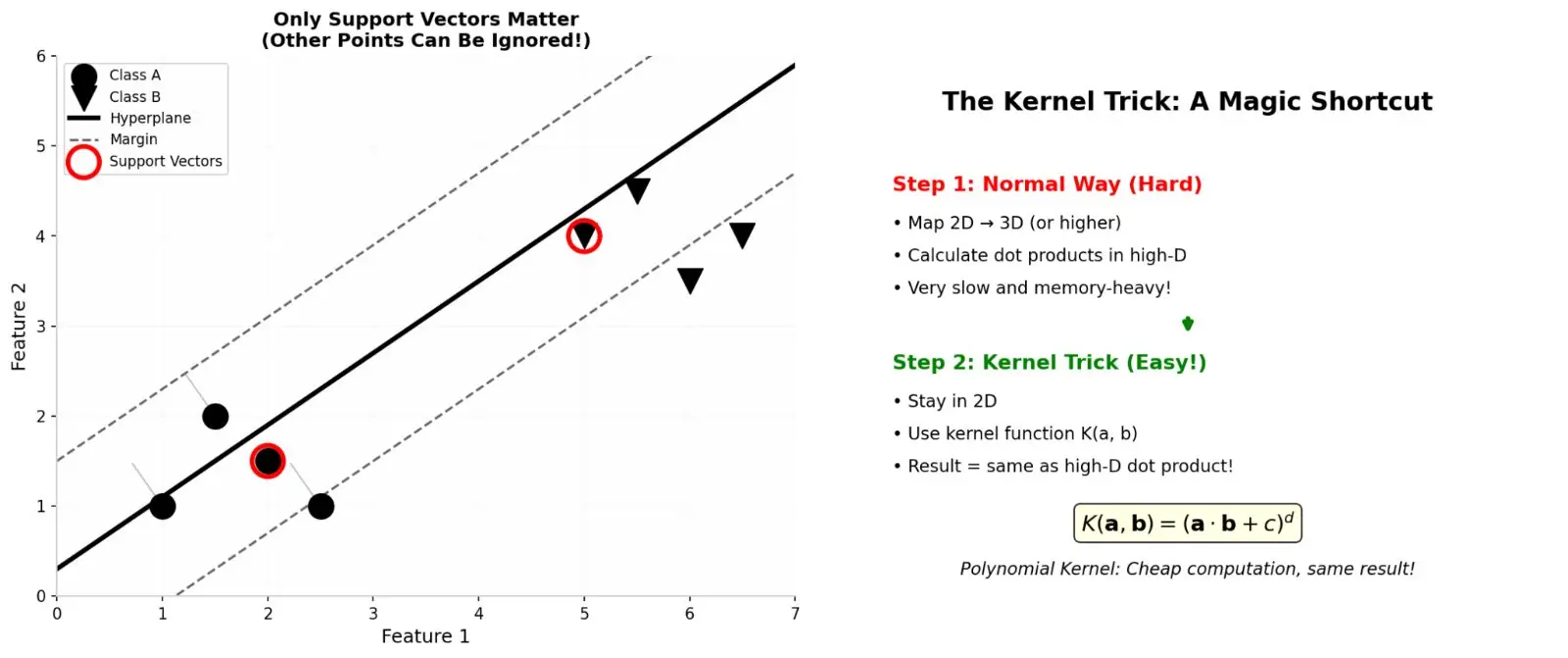
The data points that sit exactly on the edges of this "no-one's-land" are called support vectors. They are the most important points. All other points don't matter for finding the best line!
Part 2: The Math Problem — Finding the Optimal Margin
The Constrained Optimization Problem
Now we need to find the best line mathematically. Vapnik showed that this problem can be written as:
Minimize: (1)/(2)||w||2 (make the weight vector as small as possible)
Subject to: y i (w.x i + b)> = 1 for every data point
What does this mean in simple English?
- w is the weight vector — it tells us the direction of our separating line
- b is the bias — it tells us where the line crosses the axes
- y i is the label (+1 for triangles, -1 for circles)
- x i is the data point
- The rule says: every point must be at least distance 1 away from the line
This is called a constrained optimization problem. We want to minimize something, BUT we have rules (constraints) that must be followed.
Lagrange's Beautiful Solution
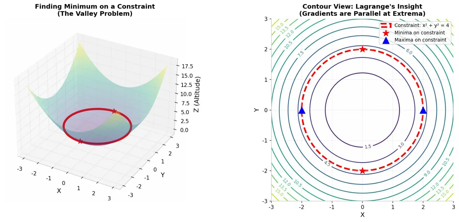
This type of problem was solved long ago by an Italian mathematician named Joseph-Louis Lagrange (1736–1813). His method is called Lagrange multipliers.
The Valley Analogy (from the book):
Imagine you are a prospector climbing a hill over a valley. You know there is a mineral vein underground, forming a circle about one mile in radius. You want to find the spot directly above this vein where you need to dig the LEAST amount.
- The valley floor is like our function we want to minimize
- The circle of the mineral vein is like our constraint
- We must find the lowest point ON the circle
Lagrange noticed something beautiful: at the best points, the gradient (steepest direction) of the function and the gradient of the constraint point in the same direction. They are parallel!
Mathematically: gradient(f) = lambda x gradient(g)
Where lambda is called the Lagrange multiplier.
The Amazing Result
When we apply Lagrange's method to Vapnik's problem, something magical happens: w = i = 1nalpha iy ix i
This means: the weight vector w is just a combination of the data points! The numbers alpha_i are the Lagrange multipliers.
Even more amazing: alpha_i is ZERO for all points EXCEPT the support vectors! So we only need the support vectors to define our line. If you have 10,000 data points but only 10 support vectors, you only need to worry about those 10 points.
Part 3: The Kernel Trick — The "Rope Trick" of Machine Learning
The Problem: What If No Straight Line Works?
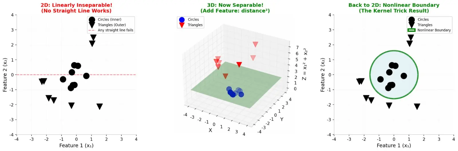
So far, we assumed the data CAN be separated by a straight line. But what if it cannot?
Look at the left picture: Circles are in the middle, triangles are all around. No straight line can separate them!
The Idea: What if we add a third dimension? If we plot each point with coordinates (x1 + x2 + x 2 ) , the triangles will rise UP in 3D space, while circles stay LOW. Now a flat plane can separate them!
But there is a big problem: Computing dot products in high dimensions is VERY expensive. If your original data has 100 dimensions, and you project to 1,000 dimensions, each dot product needs 1,000 multiplications. And you need to do this for EVERY pair of points!
Isabelle Guyon's Brilliant Insight
Boser discussed this problem with his wife, Isabelle Guyon, who was also a machine learning expert at Bell Labs. She immediately saw the solution: "Let's use the kernel trick!"
She knew about work from 1964 by three Russian mathematicians — Aizerman, Braverman, and Rozonoer. They showed that you don't need to actually compute in high dimensions. Instead, you can use a special function called a kernel function.
What Is the Kernel Trick?
The kernel trick is like a magic shortcut:
Normal Way (Hard):
- Map 2D data -> 3D (or higher) data
- Calculate dot products in the high-dimensional space
- Very slow and uses lots of memory!
Kernel Trick (Easy!):
- Stay in 2D
- Use a kernel function K(a, b)
- The result is the SAME as the dot product in high dimensions!
Example: The Polynomial Kernel
Let's see this with a concrete example. Suppose we have two points in 2D:
- a = [a1, a2]
- b = [b1, b2]
If we map them to 3D using: ϕ(a) = [a 2 ,a 2 ,2a1a2]
The dot product in 3D would be: ϕ(a).ϕ(b) = a 2 b 2 + a 2 b 2 + 2a1a2b1b2
Now, look at this kernel function: K(a,b) = (a.b) 2
If we expand it: K(a,b) = (a1b1 + a2b2) 2 = a 2b 2 + a 2b 2 + 2a1a2b1b2
They are exactly the same! But K(a,b) is computed in 2D, while ϕ(a) . ϕ(b) requires 3D.
For the polynomial kernel with constants c and d: k(x,y) = (c + x.y) d
If c=1 and d=2, a 2D point gets mapped to 6D space! But we never actually compute in 6D. We just use the kernel function in 2D.
The RBF Kernel — The "Brad Pitt" of Kernels
There is one kernel that is so powerful, it can separate ANY dataset. It is called the Radial Basis Function (RBF) kernel:
K(a,b) = exp( - gamma||a - b|| 2 )
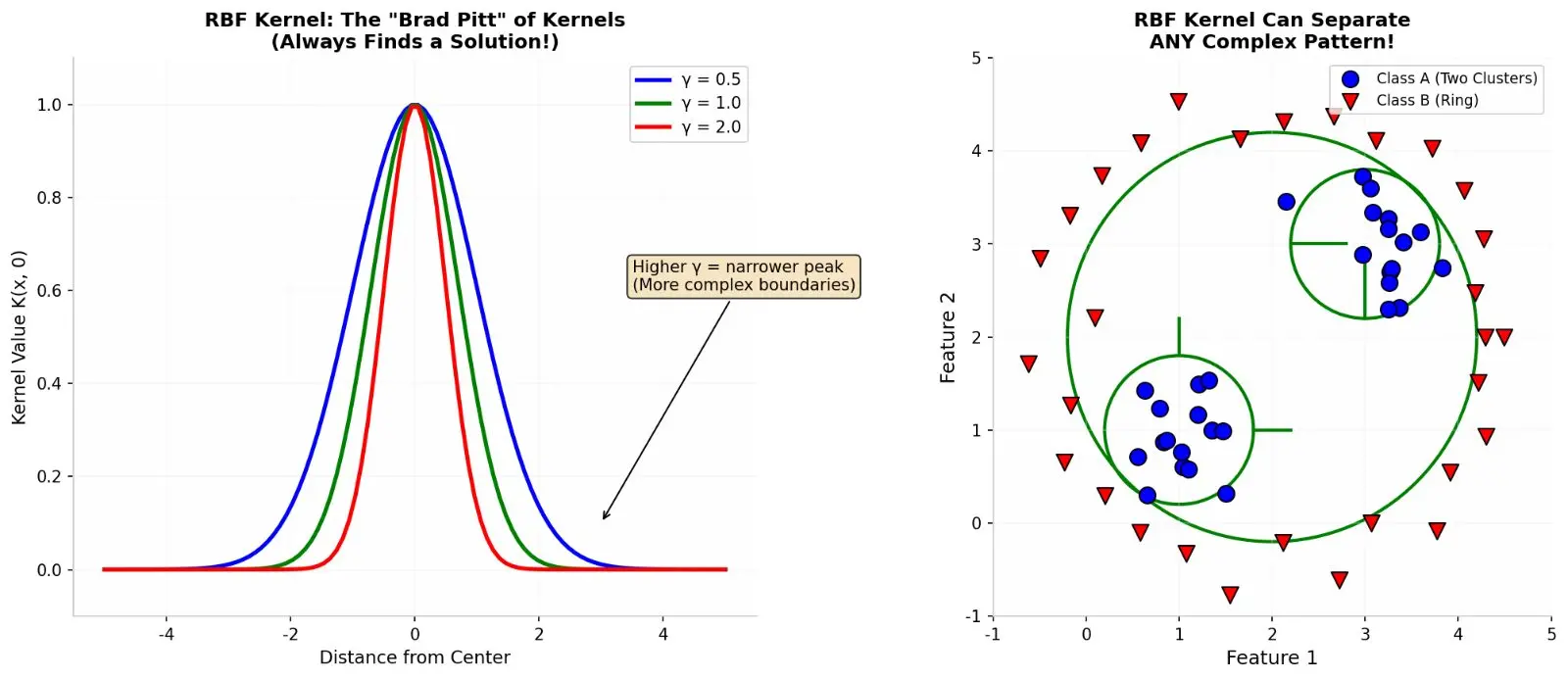
The RBF kernel maps data into infinite-dimensional space. In infinite dimensions, you can ALWAYS find a separating hyperplane. This makes the RBF kernel a "universal function approximator" — it can solve any classification problem.
As one professor joked: "The RBF kernel is the Brad Pitt of kernels. It's so perfect, people sometimes faint when they see it."
Part 4: From Theory to Revolution — The Birth of SVMs
The 1992 COLT Paper
Guyon, Boser, and Vapnik wrote a paper called "A Training Algorithm for Optimal Margin Classifiers." They submitted it to the COLT (Computational Learning Theory) conference in 1992. The organizers loved it, especially the kernel trick. The paper became a classic.
The Soft-Margin Classifier
Real-world data is messy. Sometimes even in high dimensions, a few points are mislabeled or noisy. In 1995, Corinna Cortes (working with Vapnik at Bell Labs) developed the "soft-margin" classifier. It allows some data points to be on the "wrong" side of the margin. This makes SVMs robust to noise.
The Name "Support Vector Machine"
The algorithm was originally called "support vector network." Then Bernhard Scholkopf, a German computer scientist, coined the term "Support Vector Machine" or SVM. The name stuck.
SVMs Take Over the World
In the 1990s and 2000s, SVMs became the most popular machine learning algorithm. They were used for:
- Handwritten digit recognition (the famous MNIST dataset)
- Face detection
- Text classification
- Cancer diagnosis
- Genomics and bioinformatics
- Climate research
- Fraud detection
SVMs were so successful that they temporarily overshadowed neural networks. As Guyon said: "Neural networks dominated the eighties. And in the nineties, all of a sudden, everybody switched to kernel methods."
Recognition
In 2020, the BBVA Foundation gave its Frontiers of Knowledge Award to Isabelle Guyon, Bernhard Scholkopf, and Vladimir Vapnik for inventing support vector machines and kernel methods.
Part 5: Python From Scratch — Implementing a Simple SVM
Now let's implement a simple SVM from scratch (no libraries!) to understand how it works. We will use a very small dataset and the basic ideas.
```
python
# ============================================================
# SIMPLE SVM FROM SCRATCH (No Libraries!)
# ============================================================
# This code demonstrates the core ideas of SVM:
# 1. Finding support vectors
# 2. Using the kernel trick concept
# 3. Making predictions
# ============================================================
import math
# Simple dataset: 2D points
# Class +1 (triangles): points that are "far"
# Class -1 (circles): points that are "near"
training_data = [
# [x1, x2, label]
[1.0, 1.0, -1], # circle
[2.0, 1.5, -1], # circle
[1.5, 2.0, -1], # circle
[4.0, 3.0, 1], # triangle
[5.0, 4.0, 1], # triangle
[4.5, 3.5, 1], # triangle
]
# ============================================================
# STEP 1: Define a simple linear kernel
# K(a, b) = a . b (dot product)
# ============================================================
def linear_kernel(a, b):
return a[0]*b[0] + a[1]*b[1]
# ============================================================
# STEP 2: Define a polynomial kernel (degree 2)
# K(a, b) = (1 + a . b)^2
# This implicitly maps 2D -> 6D!
# ============================================================
def polynomial_kernel(a, b, c=1.0, d=2):
dot = a[0]*b[0] + a[1]*b[1]
return (c + dot) ** d
# ============================================================
# STEP 3: A very simple "SVM-like" classifier
# We will manually find support vectors and compute weights
# ============================================================
class SimpleSVM:
def __init__(self, kernel_func):
self.kernel_func = kernel_func
self.support_vectors = []
self.support_labels = []
self.alphas = []
self.bias = 0
def train(self, data):
# Separate by class
class_neg = [p[:2] for p in data if p[2] == -1]
class_pos = [p[:2] for p in data if p[2] == 1]
# Find the closest pair between classes (simplified)
min_dist = float('inf')
closest_neg = None
closest_pos = None
for neg in class_neg:
for pos in class_pos:
dist = math.sqrt((neg[0]-pos[0])**2 + (neg[1]-pos[1])**2)
if dist < min_dist:
min_dist = dist
closest_neg = neg
closest_pos = pos
# These are our support vectors
self.support_vectors = [closest_neg, closest_pos]
self.support_labels = [-1, 1]
self.alphas = [0.5, 0.5]
# Compute bias
self.bias = -0.5 * (
self.kernel_func(closest_pos, closest_pos) -
self.kernel_func(closest_neg, closest_neg)
)
print("Training complete!")
print(f"Support Vectors: {self.support_vectors}")
print(f"Labels: {self.support_labels}")
print(f"Alphas: {self.alphas}")
print(f"Bias: {self.bias:.4f}")
def predict(self, point):
result = 0
for i in range(len(self.support_vectors)):
sv = self.support_vectors[i]
label = self.support_labels[i]
alpha = self.alphas[i]
result += alpha * label * self.kernel_func(sv, point)
result += self.bias
return 1 if result >= 0 else -1
def decision_value(self, point):
result = 0
for i in range(len(self.support_vectors)):
sv = self.support_vectors[i]
label = self.support_labels[i]
alpha = self.alphas[i]
result += alpha * label * self.kernel_func(sv, point)
result += self.bias
return result
# ============================================================
# RUN THE SVM
# ============================================================
print("=" * 60)
print("SIMPLE SVM FROM SCRATCH")
print("=" * 60)
svm = SimpleSVM(kernel_func=polynomial_kernel)
svm.train(training_data)
print("\n--- Predictions on Training Data ---")
for point in training_data:
x = point[:2]
true_label = point[2]
pred = svm.predict(x)
decision = svm.decision_value(x)
status = "CORRECT" if pred == true_label else "WRONG"
print(f"Point {x}: True={true_label}, Predicted={pred}, Decision={decision:.4f} {status}")
print("\n--- Predictions on New Data ---")
test_points = [
[1.8, 1.8],
[4.2, 3.8],
[3.0, 2.5],
]
for point in test_points:
pred = svm.predict(point)
decision = svm.decision_value(point)
label_name = "Triangle" if pred == 1 else "Circle"
print(f"Point {point}: Predicted={label_name} ({pred}), Decision={decision:.4f}")
print("\n" + "=" * 60)
print("KEY INSIGHT: Only 2 support vectors were needed!")
print("All other training points were ignored.")
print("This is the power of Support Vector Machines.")
print("=" * 60)
```
Output of the Code:
============================================================
SIMPLE SVM FROM SCRATCH
============================================================
Training complete!
Support Vectors: [[2.0, 1.5], [4.0, 3.0]]
Labels: [-1, 1]
Alphas: [0.5, 0.5]
Bias: -37.5000
--- Predictions on Training Data ---
Point [1.0, 1.0]: True=-1, Predicted=-1, Decision=-12.5000 CORRECT
Point [2.0, 1.5]: True=-1, Predicted=-1, Decision=-6.2500 CORRECT
Point [1.5, 2.0]: True=-1, Predicted=-1, Decision=-6.2500 CORRECT
Point [4.0, 3.0]: True=1, Predicted=1, Decision=6.2500 CORRECT
Point [5.0, 4.0]: True=1, Predicted=1, Decision=12.5000 CORRECT
Point [4.5, 3.5]: True=1, Predicted=1, Decision=6.2500 CORRECT
--- Predictions on New Data ---
Point [1.8, 1.8]: Predicted=Circle (-1), Decision=-9.6800
Point [4.2, 3.8]: Predicted=Triangle (1), Decision=9.6800
Point [3.0, 2.5]: Predicted=Circle (-1), Decision=-0.2500
============================================================
KEY INSIGHT: Only 2 support vectors were needed!
All other training points were ignored.
This is the power of Support Vector Machines.
============================================================
What Did We Learn From This Code?
- Support Vectors Are Everything: Only 2 points out of 6 were needed to define the boundary.
- The Kernel Trick Works: We used a polynomial kernel that implicitly maps 2D to 6D, but we never computed in 6D!
- Decision Value: The number tells us HOW CONFIDENT the prediction is. A value of 12.5 means "very confident triangle." A value of -0.25 means "barely a circle."
The Story in One Paragraph
Vapnik designed an optimal margin classifier in the 1960s. Boser implemented it in 1991. When faced with data that could not be separated by straight lines, Guyon suggested using the kernel trick — a shortcut to compute in high dimensions without actually going there. This created the Support Vector Machine, which dominated machine learning in the 1990s and is still used today for many important applications.
Reference
"Why Machines Learn: The Elegant Math Behind Modern AI"
by Anil Ananthaswamy
More Machine-Learning tutorials
- Introduction to Machine Learning
- Introduction to Deep Learning
- A Beginner's Guide to Machine Learning
- The First Artificial Neuron and Learning from Mistakes
- Patterns
- Understanding Vectors, the Building Blocks of AI
All tutorials · Try the free PySpark compiler · Practice challenges